Introduction Computer Science & Engineering 423/823 Design and - - PDF document

SLIDE 1

Computer Science & Engineering 423/823 Design and Analysis of Algorithms

Lecture 06 — Dynamic Programming (Chapter 15) Stephen Scott (Adapted from Vinodchandran N. Variyam) sscott@cse.unl.edu

Introduction

I Dynamic programming is a technique for solving optimization problems I Key element: Decompose a problem into subproblems, solve them

recursively, and then combine the solutions into a final (optimal) solution

I Important component: There are typically an exponential number of

subproblems to solve, but many of them overlap

) Can re-use the solutions rather than re-solving them

I Number of distinct subproblems is polynomial

Rod Cutting (1)

I A company has a rod of length n and wants to cut it into smaller rods to

maximize profit

I Have a table telling how much they get for rods of various lengths: A

rod of length i has price pi

I The cuts themselves are free, so profit is based solely on the prices

charged for of the rods

I If cuts only occur at integral boundaries 1, 2, . . . , n 1, then can make

• r not make a cut at each of n 1 positions, so total number of possible

solutions is 2n1

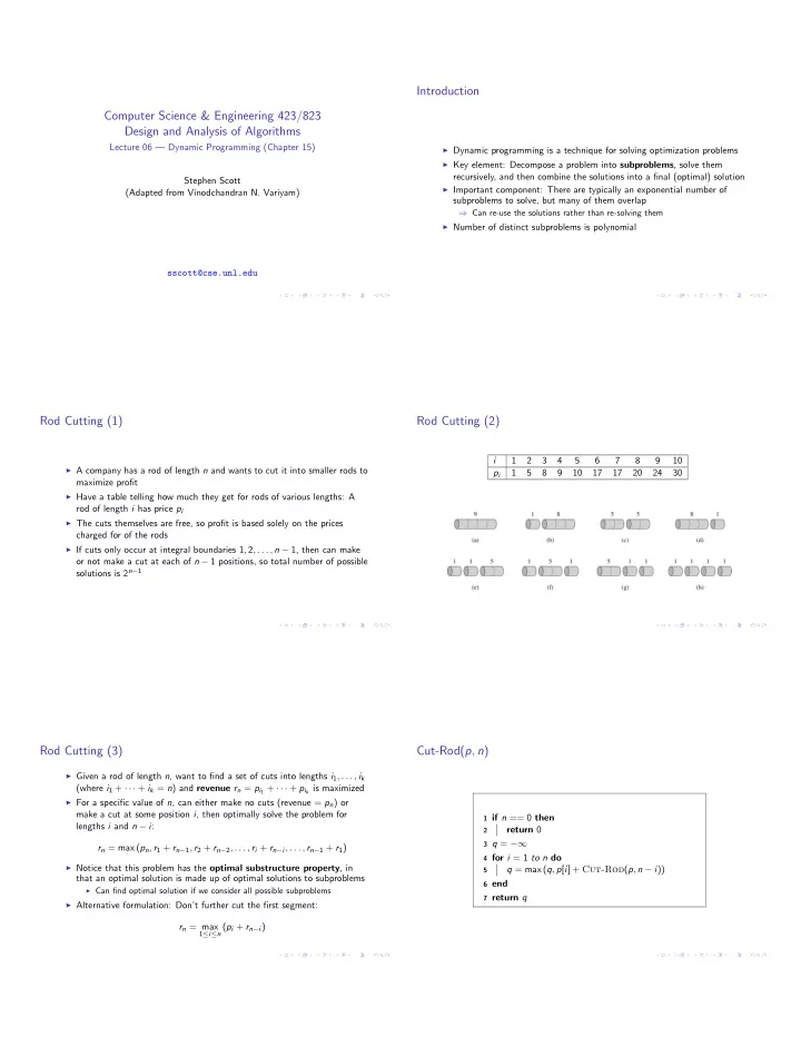
Rod Cutting (2)

i 1 2 3 4 5 6 7 8 9 10 pi 1 5 8 9 10 17 17 20 24 30

Rod Cutting (3)

I Given a rod of length n, want to find a set of cuts into lengths i1, . . . , ik

(where i1 + · · · + ik = n) and revenue rn = pi1 + · · · + pik is maximized

I For a specific value of n, can either make no cuts (revenue = pn) or

make a cut at some position i, then optimally solve the problem for lengths i and n i: rn = max (pn, r1 + rn1, r2 + rn2, . . . , ri + rni, . . . , rn1 + r1)

I Notice that this problem has the optimal substructure property, in

that an optimal solution is made up of optimal solutions to subproblems

I Can find optimal solution if we consider all possible subproblems

I Alternative formulation: Don’t further cut the first segment:

rn = max

1in (pi + rni)

Cut-Rod(p, n)

1 if n == 0 then 2

return 0

3 q = 1 4 for i = 1 to n do 5

q = max (q, p[i] + Cut-Rod(p, n i))

6 end 7 return q

SLIDE 2

Time Complexity

I Let T(n) be number of calls to Cut-Rod I Thus T(0) = 1 and, based on the for loop,

T(n) = 1 +

n1

X

j=0

T(j) = 2n

I Why exponential? Cut-Rod exploits the optimal substructure property,

but repeats work on these subproblems

I E.g., if the first call is for n = 4, then there will be:

I 1 call to Cut-Rod(4) I 1 call to Cut-Rod(3) I 2 calls to Cut-Rod(2) I 4 calls to Cut-Rod(1) I 8 calls to Cut-Rod(0)

Time Complexity (2)

Recursion Tree for n = 4

Dynamic Programming Algorithm

I Can save time dramatically by remembering results from prior calls I Two general approaches:

• 1. Top-down with memoization: Run the recursive algorithm as defined

earlier, but before recursive call, check to see if the calculation has already been done and memoized

• 2. Bottom-up: Fill in results for “small” subproblems first, then use these to

fill in table for “larger” ones

I Typically have the same asymptotic running time

Memoized-Cut-Rod-Aux(p, n, r)

1 if r[n] 0 then 2

return r[n] // r initialized to all 1

3 if n == 0 then 4

q = 0

5 else 6

q = 1

7

for i = 1 to n do

8

q = max (q, p[i] + Memoized-Cut-Rod-Aux(p, n i, r))

9

end

10

r[n] = q

11 return q

Bottom-Up-Cut-Rod(p, n)

1 Allocate r[0 . . . n] 2 r[0] = 0 3 for j = 1 to n do 4

q = 1

5

for i = 1 to j do

6

q = max (q, p[i] + r[j i])

7

end

8

r[j] = q

9 end 10 return r[n]

First solves for n = 0, then for n = 1 in terms of r[0], then for n = 2 in terms

• f r[0] and r[1], etc.

Example

i 1 2 3 4 5 6 7 8 9 10 pi 1 5 8 9 10 17 17 20 24 30 j = 1 j = 4 i = 1 p1 + r0 = 1 = r1 i = 1 p1 + r3 = 1 + 8 = 9 j = 2 i = 2 p2 + r2 = 5 + 5 = 10 = r4 i = 1 p1 + r1 = 2 i = 3 p3 + r1 + 8 + 1 = 9 i = 2 p2 + r0 = 5 = r2 i = 4 p4 + r0 = 9 + 0 = 9 j = 3 i = 1 p1 + r2 = 1 + 5 = 6 i = 2 p2 + r1 = 5 + 1 = 6 i = 3 p3 + r0 = 8 + 0 = 8 = r3

SLIDE 3

Time Complexity

Subproblem graph for n = 4 Both algorithms take linear time to solve for each value of n, so total time complexity is Θ(n2)

Reconstructing a Solution

I If interested in the set of cuts for an optimal solution as well as the

revenue it generates, just keep track of the choice made to optimize each subproblem

I Will add a second array s, which keeps track of the optimal size of the

first piece cut in each subproblem

Extended-Bottom-Up-Cut-Rod(p, n)

1 Allocate r[0 . . . n] and s[0 . . . n] 2 r[0] = 0 3 for j = 1 to n do 4

q = 1

5

for i = 1 to j do

6

if q < p[i] + r[j i] then

7

q = p[i] + r[j i]

8

s[j] = i

9 10

end

11

r[j] = q

12 end 13 return r, s

Print-Cut-Rod-Solution(p, n)

1 (r, s) = Extended-Bottom-Up-Cut-Rod(p, n) 2 while n > 0 do 3

print s[n]

4

n = n s[n]

5 end

Example: i 1 2 3 4 5 6 7 8 9 10 r[i] 1 5 8 10 13 17 18 22 25 30 s[i] 1 2 3 2 2 6 1 2 3 10 If n = 10, optimal solution is no cut; if n = 7, then cut once to get segments

• f sizes 1 and 6

Matrix-Chain Multiplication (1)

I Given a chain of matrices hA1, . . . , Ani, goal is to compute their product

A1 · · · An

I This operation is associative, so can sequence the multiplications in

multiple ways and get the same result

I Can cause dramatic changes in number of operations required I Multiplying a p ⇥ q matrix by a q ⇥ r matrix requires pqr steps and

yields a p ⇥ r matrix for future multiplications

I E.g., Let A1 be 10 ⇥ 100, A2 be 100 ⇥ 5, and A3 be 5 ⇥ 50

• 1. Computing ((A1A2)A3) requires 10 · 100 · 5 = 5000 steps to compute

(A1A2) (yielding a 10 ⇥ 5), and then 10 · 5 · 50 = 2500 steps to finish, for a total of 7500

• 2. Computing (A1(A2A3)) requires 100 · 5 · 50 = 25000 steps to compute

(A2A3) (yielding a 100 ⇥ 50), and then 10 · 100 · 50 = 50000 steps to finish, for a total of 75000

Matrix-Chain Multiplication (2)

I The matrix-chain multiplication problem is to take a chain

hA1, . . . , Ani of n matrices, where matrix i has dimension pi1 ⇥ pi, and fully parenthesize the product A1 · · · An so that the number of scalar multiplications is minimized

I Brute force solution is infeasible, since its time complexity is Ω

• 4n/n3/2

I Will follow 4-step procedure for dynamic programming:

• 1. Characterize the structure of an optimal solution
• 2. Recursively define the value of an optimal solution
• 3. Compute the value of an optimal solution
• 4. Construct an optimal solution from computed information

SLIDE 4

Characterizing the Structure of an Optimal Solution

I Let Ai...j be the matrix from the product AiAi+1 · · · Aj I To compute Ai...j, must split the product and compute Ai...k and Ak+1...j

for some integer k, then multiply the two together

I Cost is the cost of computing each subproduct plus cost of multiplying

the two results

I Say that in an optimal parenthesization, the optimal split for

AiAi+1 · · · Aj is at k

I Then in an optimal solution for AiAi+1 · · · Aj, the parenthisization of

Ai · · · Ak is itself optimal for the subchain Ai · · · Ak (if not, then we could do better for the larger chain)

I Similar argument for Ak+1 · · · Aj I Thus if we make the right choice for k and then optimally solve the

subproblems recursively, we’ll end up with an optimal solution

I Since we don’t know optimal k, we’ll try them all

Recursively Defining the Value of an Optimal Solution

I Define m[i, j] as minimum number of scalar multiplications needed to

compute Ai...j

I (What entry in the m table will be our final answer?) I Computing m[i, j]:

• 1. If i = j, then no operations needed and m[i, i] = 0 for all i
• 2. If i < j and we split at k, then optimal number of operations needed is the
• ptimal number for computing Ai...k and Ak+1...j, plus the number to

multiply them: m[i, j] = m[i, k] + m[k + 1, j] + pi1pkpj

• 3. Since we don’t know k, we’ll try all possible values:

m[i, j] = ⇢ if i = j minik<j{m[i, k] + m[k + 1, j] + pi1pkpj} if i < j

I To track the optimal solution itself, define s[i, j] to be the value of k

used at each split

Computing the Value of an Optimal Solution

I As with the rod cutting problem, many of the subproblems we’ve defined

will overlap

I Exploiting overlap allows us to solve only Θ(n2) problems (one problem

for each (i, j) pair), as opposed to exponential

I We’ll do a bottom-up implementation, based on chain length I Chains of length 1 are trivially solved (m[i, i] = 0 for all i) I Then solve chains of length 2, 3, etc., up to length n I Linear time to solve each problem, quadratic number of problems, yields

O(n3) total time

Matrix-Chain-Order(p, n)

1 allocate m[1 . . . n, 1 . . . n] and s[1 . . . n, 1 . . . n] 2 initialize m[i, i] = 0 8 1  i  n 3 for ` = 2 to n do 4

for i = 1 to n ` + 1 do

5

j = i + ` 1

6

m[i, j] = 1

7

for k = i to j 1 do

8

q = m[i, k] + m[k + 1, j] + pi−1pkpj

9

if q < m[i, j] then

10

m[i, j] = q

11

s[i, j] = k

12 13

end

14

end

15 end 16 return (m, s)

Example

matrix A1 A2 A3 A4 A5 A6 dimension 30 ⇥ 35 35 ⇥ 15 15 ⇥ 5 5 ⇥ 10 10 ⇥ 20 20 ⇥ 25

Constructing an Optimal Solution from Computed Information

I Cost of optimal parenthesization is stored in m[1, n] I First split in optimal parenthesization is between s[1, n] and s[1, n] + 1 I Descending recursively, next splits are between s[1, s[1, n]] and

s[1, s[1, n]] + 1 for left side and between s[s[1, n] + 1, n] and s[s[1, n] + 1, n] + 1 for right side

I and so on...

SLIDE 5

Print-Optimal-Parens(s, i, j)

1 if i == j then 2

print “A”i

3 else 4

print “(”

5

Print-Optimal-Parens(s, i, s[i, j])

6

Print-Optimal-Parens(s, s[i, j] + 1, j)

7

print “)”

8

Example

Optimal parenthesization: ((A1(A2A3))((A4A5)A6))

Example of How Subproblems Overlap

Entire subtrees overlap: See Section 15.3 for more on optimal substructure and overlapping subproblems

Longest Common Subsequence

I Sequence Z = hz1, z2, . . . , zki is a subsequence of another sequence

X = hx1, x2, . . . , xmi if there is a strictly increasing sequence hi1, . . . , iki

• f indices of X such that for all j = 1, . . . , k, xij = zj

I I.e., as one reads through Z, one can find a match to each symbol of Z

in X, in order (though not necessarily contiguous)

I E.g., Z = hB, C, D, Bi is a subsequence of X = hA, B, C, B, D, A, Bi

since z1 = x2, z2 = x3, z3 = x5, and z4 = x7

I Z is a common subsequence of X and Y if it is a subsequence of both I The goal of the longest common subsequence problem is to find a

maximum-length common subsequence (LCS) of sequences X = hx1, x2, . . . , xmi and Y = hy1, y2, . . . , yni

Characterizing the Structure of an Optimal Solution

I Given sequence X = hx1, . . . , xmi, the ith prefix of X is Xi = hx1, . . . , xii I Theorem If X = hx1, . . . , xmi and Y = hy1, . . . , yni have LCS

Z = hz1, . . . , zki, then

• 1. xm = yn ) zk = xm = yn and Zk1 is LCS of Xm1 and Yn1

I If zk 6= xm, can lengthen Z, ) contradiction I If Zk−1 not LCS of Xm−1 and Yn−1, then a longer CS of Xm−1 and Yn−1

could have xm appended to it to get CS of X and Y that is longer than Z, ) contradiction

• 2. If xm 6= yn, then zk 6= xm implies that Z is an LCS of Xm1 and Y

I If zk 6= xm, then Z is a CS of Xm−1 and Y . Any CS of Xm−1 and Y that is

longer than Z would also be a longer CS for X and Y , ) contradiction

• 3. If xm 6= yn, then zk 6= yn implies that Z is an LCS of X and Yn1

I Similar argument to (2)

Recursively Defining the Value of an Optimal Solution

I The theorem implies the kinds of subproblems that we’ll investigate to

find LCS of X = hx1, . . . , xmi and Y = hy1, . . . , yni

I If xm = yn, then find LCS of Xm1 and Yn1 and append xm (= yn) to it I If xm 6= yn, then find LCS of X and Yn1 and find LCS of Xm1 and Y

and identify the longest one

I Let c[i, j] = length of LCS of Xi and Yj

c[i, j] = 8 < : if i = 0 or j = 0 c[i 1, j 1] + 1 if i, j > 0 and xi = yj max (c[i, j 1], c[i 1, j]) if i, j > 0 and xi 6= yj

SLIDE 6

LCS-Length(X, Y , m, n)

1 allocate b[1 . . . m, 1 . . . n] and c[0 . . . m, 0 . . . n] 2 initialize c[i, 0] = 0 and c[0, j] = 0 8 0  i  m and 0  j  n 3 for i = 1 to m do 4

for j = 1 to n do

5

if xi == yj then

6

c[i, j] = c[i 1, j 1] + 1

7

b[i, j] = “ - ”

8

else if c[i 1, j] c[i, j 1] then

9

c[i, j] = c[i 1, j]

10

b[i, j] = “ " ”

11

else

12

c[i, j] = c[i, j 1]

13

b[i, j] = “ ”

14 15

end

16 end 17 return (c, b)

What is the time complexity?

Example

X = hA, B, C, B, D, A, Bi, Y = hB, D, C, A, B, Ai

Constructing an Optimal Solution from Computed Information

I Length of LCS is stored in c[m, n] I To print LCS, start at b[m, n] and follow arrows until in row or column 0 I If in cell (i, j) on this path, when xi = yj (i.e., when arrow is “ - ”),

print xi as part of the LCS

I This will print LCS backwards

Print-LCS(b, X, i, j)

1 if i == 0 or j == 0 then 2

return

3 if b[i, j] == “ - ” then 4

Print-LCS(b, X, i 1, j 1)

5

print xi

6 else if b[i, j] == “ " ” then 7

Print-LCS(b, X, i 1, j)

8 else Print-LCS(b, X, i, j 1)

What is the time complexity?

Example

X = hA, B, C, B, D, A, Bi, Y = hB, D, C, A, B, Ai, prints “BCBA”

Optimal Binary Search Trees

I Goal is to construct binary search trees such that most frequently sought

values are near the root, thus minimizing expected search time

I Given a sequence K = hk1, . . . , kni of n distinct keys in sorted order I Key ki has probability pi that it will be sought on a particular search I To handle searches for values not in K, have n + 1 dummy keys

d0, d1, . . . , dn to serve as the tree’s leaves

I Dummy key di will be reached with probability qi I If depthT(ki) is distance from root of ki in tree T, then expected search

cost of T is 1 +

n

X

i=1

pi depthT(ki) +

n

X

i=0

qi depthT(di)

I An optimal binary search tree is one with minimum expected search

cost

SLIDE 7

Optimal Binary Search Trees (2)

i 1 2 3 4 5 pi 0.15 0.10 0.05 0.10 0.20 qi 0.05 0.10 0.05 0.05 0.05 0.10

expected cost = 2.80 expected cost = 2.75 (optimal)

Characterizing the Structure of an Optimal Solution

I Observation: Since K is sorted and dummy keys interspersed in order,

any subtree of a BST must contain keys in a contiguous range ki, . . . , kj and have leaves di1, . . . , dj

I Thus, if an optimal BST T has a subtree T 0 over keys ki, . . . , kj, then

T 0 is optimal for the subproblem consisting of only the keys ki, . . . , kj

I If T 0 weren’t optimal, then a lower-cost subtree could replace T 0 in T, )

contradiction

I Given keys ki, . . . , kj, say that its optimal BST roots at kr for some

i  r  j

I Thus if we make right choice for kr and optimally solve the problem for

ki, . . . , kr1 (with dummy keys di1, . . . , dr1) and the problem for kr+1, . . . , kj (with dummy keys dr, . . . , dj), we’ll end up with an optimal solution

I Since we don’t know optimal kr, we’ll try them all

Recursively Defining the Value of an Optimal Solution

I Define e[i, j] as the expected cost of searching an optimal BST built on

keys ki, . . . , kj

I If j = i 1, then there is only the dummy key di1, so e[i, i 1] = qi1 I If j i, then choose root kr from ki, . . . , kj and optimally solve

subproblems ki, . . . , kr1 and kr+1, . . . , kj

I When combining the optimal trees from subproblems and making them

children of kr, we increase their depth by 1, which increases the cost of each by the sum of the probabilities of its nodes

I Define w(i, j) = Pj `=i p` + Pj `=i1 q` as the sum of probabilities of the

nodes in the subtree built on ki, . . . , kj, and get e[i, j] = pr + (e[i, r 1] + w(i, r 1)) + (e[r + 1, j] + w(r + 1, j))

Recursively Defining the Value of an Optimal Solution (2)

I Note that

w(i, j) = w(i, r 1) + pr + w(r + 1, j)

I Thus we can condense the equation to

e[i, j] = e[i, r 1] + e[r + 1, j] + w(i, j)

I Finally, since we don’t know what kr should be, we try them all:

e[i, j] = ⇢ qi1 if j = i 1 minirj{e[i, r 1] + e[r + 1, j] + w(i, j)} if i  j

I Will also maintain table root[i, j] = index r for which kr is root of an

• ptimal BST on keys ki, . . . , kj

Optimal-BST(p, q, n)

1 allocate e[1 . . . n + 1, 0 . . . n], w[1 . . . n + 1, 0 . . . n], and root[1 . . . n, 1 . . . n] 2 initialize e[i, i − 1] = w[i, i − 1] = qi−1 ∀ 1 ≤ i ≤ n + 1 3 for ` = 1 to n do 4 for i = 1 to n − ` + 1 do 5 j = i + ` − 1 6 e[i, j] = ∞ 7 w[i, j] = w[i, j − 1] + pj + qj 8 for r = i to j do 9 t = e[i, r − 1] + e[r + 1, j] + w[i, j] 10 if t < e[i, j] then 11 e[i, j] = t 12 root[i, j] = r 13 14 end 15 end 16 end 17 return (e, root)

What is the time complexity?

Example

i 1 2 3 4 5 pi 0.15 0.10 0.05 0.10 0.20 qi 0.05 0.10 0.05 0.05 0.05 0.10