Introduction CSCE423/823 CSCE423/823 Given a weighted, directed - - PDF document

SLIDE 1 CSCE423/823 Introduction Bellman-Ford Algorithm SSSPs in Directed Acyclic Graphs Dijkstra’s Algorithm Difference Constraints and Shortest Paths

Computer Science & Engineering 423/823 Design and Analysis of Algorithms

Lecture 05 — Single-Source Shortest Paths (Chapter 24) Stephen Scott (Adapted from Vinodchandran N. Variyam)

1 / 36 CSCE423/823 Introduction Optimal Substructure of a Shortest Path Negative-Weight Edges Cycles Relaxation Bellman-Ford Algorithm SSSPs in Directed Acyclic Graphs Dijkstra’s Algorithm Difference Constraints and Shortest Paths

Introduction

Given a weighted, directed graph G = (V, E) with weight function w : E ! R The weight of path p = hv0, v1, . . . , vki is the sum of the weights of its edges: w(p) =

k

X

i=1

w(vi−1, vi) Then the shortest-path weight from u to v is (u, v) = ⇢ min{w(p) : u

p

v} if there is a path from u to v 1

• therwise

A shortest path from u to v is any path p with weight w(p) = (u, v) Applications: Network routing, driving directions

2 / 36 CSCE423/823 Introduction Optimal Substructure of a Shortest Path Negative-Weight Edges Cycles Relaxation Bellman-Ford Algorithm SSSPs in Directed Acyclic Graphs Dijkstra’s Algorithm Difference Constraints and Shortest Paths

Types of Shortest Path Problems

Given G as described earlier, Single-Source Shortest Paths: Find shortest paths from source node s to every other node Single-Destination Shortest Paths: Find shortest paths from every node to destination t

Can solve with SSSP solution. How?

Single-Pair Shortest Path: Find shortest path from specific node u to specific node v

Can solve via SSSP; no asymptotically faster algorithm known

All-Pairs Shortest Paths: Find shortest paths between every pair of nodes

Can solve via repeated application of SSSP, but can do better

3 / 36 CSCE423/823 Introduction Optimal Substructure of a Shortest Path Negative-Weight Edges Cycles Relaxation Bellman-Ford Algorithm SSSPs in Directed Acyclic Graphs Dijkstra’s Algorithm Difference Constraints and Shortest Paths

Optimal Substructure of a Shortest Path

The shortest paths problem has the optimal substructure property: If p = hv0, v1, . . . , vki is a SP from v0 to vk, then for 0  i  j  k, pij = hvi, vi+1, . . . , vji is a SP from vi to vj

Proof: Let p = v0

p0i

vi

pij

vj

pjk

vk with weight w(p) = w(p0i) + w(pij) + w(pjk). If there exists a path p0

ij from vi to

vj with w(p0

ij) < w(pij), then p is not a SP since

v0

p0i

vi

p0

ij

vj

pjk

vk has less weight than p

This property helps us to use a greedy algorithm for this problem

4 / 36 CSCE423/823 Introduction Optimal Substructure of a Shortest Path Negative-Weight Edges Cycles Relaxation Bellman-Ford Algorithm SSSPs in Directed Acyclic Graphs Dijkstra’s Algorithm Difference Constraints and Shortest Paths

Negative-Weight Edges (1)

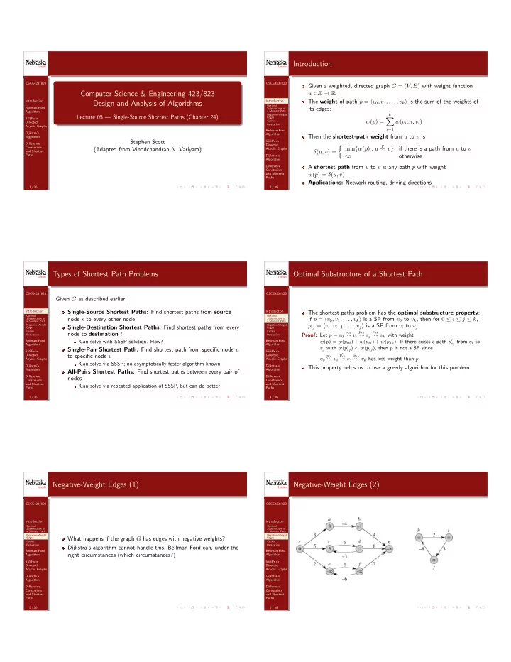
What happens if the graph G has edges with negative weights? Dijkstra’s algorithm cannot handle this, Bellman-Ford can, under the right circumstances (which circumstances?)

5 / 36 CSCE423/823 Introduction Optimal Substructure of a Shortest Path Negative-Weight Edges Cycles Relaxation Bellman-Ford Algorithm SSSPs in Directed Acyclic Graphs Dijkstra’s Algorithm Difference Constraints and Shortest Paths

Negative-Weight Edges (2)

6 / 36

SLIDE 2 CSCE423/823 Introduction Optimal Substructure of a Shortest Path Negative-Weight Edges Cycles Relaxation Bellman-Ford Algorithm SSSPs in Directed Acyclic Graphs Dijkstra’s Algorithm Difference Constraints and Shortest Paths

Cycles

What kinds of cycles might appear in a shortest path?

Negative-weight cycle Zero-weight cycle Positive-weight cycle

7 / 36 CSCE423/823 Introduction Optimal Substructure of a Shortest Path Negative-Weight Edges Cycles Relaxation Bellman-Ford Algorithm SSSPs in Directed Acyclic Graphs Dijkstra’s Algorithm Difference Constraints and Shortest Paths

Relaxation

Given weighted graph G = (V, E) with source node s 2 V and other node v 2 V (v 6= s), we’ll maintain d[v], which is upper bound on (s, v) Relaxation of an edge (u, v) is the process of testing whether we can decrease d[v], yielding a tighter upper bound

8 / 36 CSCE423/823 Introduction Optimal Substructure of a Shortest Path Negative-Weight Edges Cycles Relaxation Bellman-Ford Algorithm SSSPs in Directed Acyclic Graphs Dijkstra’s Algorithm Difference Constraints and Shortest Paths

Initialize-Single-Source(G, s)

for each vertex v 2 V do

1

d[v] = 1

2

⇡[v] = nil

3 end 4 d[s] = 0

How is the invariant maintained?

9 / 36 CSCE423/823 Introduction Optimal Substructure of a Shortest Path Negative-Weight Edges Cycles Relaxation Bellman-Ford Algorithm SSSPs in Directed Acyclic Graphs Dijkstra’s Algorithm Difference Constraints and Shortest Paths

Relax(u, v, w)

if d[v] > d[u] + w(u, v) then

1

d[v] = d[u] + w(u, v)

2

⇡[v] = u

3

How do we know that we can tighten d[v] like this?

10 / 36 CSCE423/823 Introduction Optimal Substructure of a Shortest Path Negative-Weight Edges Cycles Relaxation Bellman-Ford Algorithm SSSPs in Directed Acyclic Graphs Dijkstra’s Algorithm Difference Constraints and Shortest Paths

Relaxation Example

Numbers in nodes are values of d

11 / 36 CSCE423/823 Introduction Bellman-Ford Algorithm Introduction The Algorithm Example Analysis SSSPs in Directed Acyclic Graphs Dijkstra’s Algorithm Difference Constraints and Shortest Paths

Bellman-Ford Algorithm

Greedy algorithm Works with negative-weight edges and detects if there is a negative-weight cycle Makes |V | 1 passes over all edges, relaxing each edge during each pass

12 / 36

SLIDE 3 CSCE423/823 Introduction Bellman-Ford Algorithm Introduction The Algorithm Example Analysis SSSPs in Directed Acyclic Graphs Dijkstra’s Algorithm Difference Constraints and Shortest Paths

Bellman-Ford(G, w, s)

Initialize-Single-Source(G, s)

1 for i = 1 to |V | − 1 do 2

for each edge (u, v) ∈ E do

3

Relax(u, v, w)

4

end

5 end 6 for each edge (u, v) ∈ E do 7

if d[v] > d[u] + w(u, v) then

8

return false // G has a negative-wt cycle

9 10 end 11 return true // G has no neg-wt cycle reachable frm

s

13 / 36 CSCE423/823 Introduction Bellman-Ford Algorithm Introduction The Algorithm Example Analysis SSSPs in Directed Acyclic Graphs Dijkstra’s Algorithm Difference Constraints and Shortest Paths

Bellman-Ford Algorithm Example (1)

Within each pass, edges relaxed in this order: (t, x), (t, y), (t, z), (x, t), (y, x), (y, z), (z, x), (z, s), (s, t), (s, y)

14 / 36 CSCE423/823 Introduction Bellman-Ford Algorithm Introduction The Algorithm Example Analysis SSSPs in Directed Acyclic Graphs Dijkstra’s Algorithm Difference Constraints and Shortest Paths

Bellman-Ford Algorithm Example (2)

Within each pass, edges relaxed in this order: (t, x), (t, y), (t, z), (x, t), (y, x), (y, z), (z, x), (z, s), (s, t), (s, y)

15 / 36 CSCE423/823 Introduction Bellman-Ford Algorithm Introduction The Algorithm Example Analysis SSSPs in Directed Acyclic Graphs Dijkstra’s Algorithm Difference Constraints and Shortest Paths

Time Complexity of Bellman-Ford Algorithm

Initialize-Single-Source takes how much time? Relax takes how much time? What is time complexity of relaxation steps (nested loops)? What is time complexity of steps to check for negative-weight cycles? What is total time complexity?

16 / 36 CSCE423/823 Introduction Bellman-Ford Algorithm Introduction The Algorithm Example Analysis SSSPs in Directed Acyclic Graphs Dijkstra’s Algorithm Difference Constraints and Shortest Paths

Correctness of Bellman-Ford Algorithm

Assume no negative-weight cycles Since no cycles appear in SPs, every SP has at most |V | 1 edges Then define sets S0, S1, . . . S|V |−1: Sk = {v 2 V : 9s

p

v s.t. (s, v) = w(p) and |p|  k} Loop invariant: After ith iteration of outer relaxation loop (Line 2), for all v 2 Si, we have d[v] = (s, v)

Can prove via induction

Implies that, after |V | 1 iterations, d[v] = (s, v) for all v 2 V = S|V |−1

17 / 36 CSCE423/823 Introduction Bellman-Ford Algorithm Introduction The Algorithm Example Analysis SSSPs in Directed Acyclic Graphs Dijkstra’s Algorithm Difference Constraints and Shortest Paths

Correctness of Bellman-Ford Algorithm (2)

Let c = hv0, v1, . . . , vk = v0i be neg-weight cycle reachable from s:

k

X

i=1

w(vi−1, vi) < 0 If algorithm incorrectly returns true, then (due to Line 8) for all nodes in the cycle (i = 1, 2, . . . , k), d[vi]  d[vi−1] + w(vi−1, vi) By summing, we get

k

X

i=1

d[vi] 

k

X

i=1

d[vi−1] +

k

X

i=1

w(vi−1, vi) Since v0 = vk, Pk

i=1 d[vi] = Pk i=1 d[vi−1]

This implies that 0  Pk

i=1 w(vi−1, vi), a contradiction

18 / 36

SLIDE 4 CSCE423/823 Introduction Bellman-Ford Algorithm SSSPs in Directed Acyclic Graphs Introduction The Algorithm Example Analysis Dijkstra’s Algorithm Difference Constraints and Shortest Paths

SSSPs in Directed Acyclic Graphs

Why did Bellman-Ford have to run |V | 1 iterations of edge relaxations? To confirm that SP information fully propagated to all nodes What if we knew that, after we relaxed an edge just once, we would be completely done with it? Can do this if G a dag and we relax edges in correct order (what

• rder?)

19 / 36 CSCE423/823 Introduction Bellman-Ford Algorithm SSSPs in Directed Acyclic Graphs Introduction The Algorithm Example Analysis Dijkstra’s Algorithm Difference Constraints and Shortest Paths

Dag-Shortest-Paths(G, w, s)

topologically sort the vertices of G

1 Initialize-Single-Source(G, s) 2 for each vertex u 2 V , taken in topo sorted

• rder do

3

for each v 2 Adj[u] do

4

Relax(u, v, w)

5

end

6 end

20 / 36 CSCE423/823 Introduction Bellman-Ford Algorithm SSSPs in Directed Acyclic Graphs Introduction The Algorithm Example Analysis Dijkstra’s Algorithm Difference Constraints and Shortest Paths

SSSP dag Example (1)

21 / 36 CSCE423/823 Introduction Bellman-Ford Algorithm SSSPs in Directed Acyclic Graphs Introduction The Algorithm Example Analysis Dijkstra’s Algorithm Difference Constraints and Shortest Paths

SSSP dag Example (2)

22 / 36 CSCE423/823 Introduction Bellman-Ford Algorithm SSSPs in Directed Acyclic Graphs Introduction The Algorithm Example Analysis Dijkstra’s Algorithm Difference Constraints and Shortest Paths

Time Complexity of SSSP in dag

Topological sort takes how much time? Initialize-Single-Source takes how much time? How many calls to Relax? What is total time complexity?

23 / 36 CSCE423/823 Introduction Bellman-Ford Algorithm SSSPs in Directed Acyclic Graphs Dijkstra’s Algorithm Introduction The Algorithm Example Analysis Difference Constraints and Shortest Paths

Dijkstra’s Algorithm

Faster than Bellman-Ford Requires all edge weights to be nonnegative Maintains set S of vertices whose final shortest path weights from s have been determined

Repeatedly select u 2 V \ S with minimum SP estimate, add u to S, and relax all edges leaving u

Uses min-priority queue

24 / 36

SLIDE 5 CSCE423/823 Introduction Bellman-Ford Algorithm SSSPs in Directed Acyclic Graphs Dijkstra’s Algorithm Introduction The Algorithm Example Analysis Difference Constraints and Shortest Paths

Dijkstra(G, w, s)

Initialize-Single-Source(G, s)

1 S = ; 2 Q = V 3 while Q 6= ; do 4

u = Extract-Min(Q)

5

S = S [ {u}

6

for each v 2 Adj[u] do

7

Relax(u, v, w)

8

end

9 end

25 / 36 CSCE423/823 Introduction Bellman-Ford Algorithm SSSPs in Directed Acyclic Graphs Dijkstra’s Algorithm Introduction The Algorithm Example Analysis Difference Constraints and Shortest Paths

Dijkstra’s Algorithm Example (1)

26 / 36 CSCE423/823 Introduction Bellman-Ford Algorithm SSSPs in Directed Acyclic Graphs Dijkstra’s Algorithm Introduction The Algorithm Example Analysis Difference Constraints and Shortest Paths

Dijkstra’s Algorithm Example (2)

27 / 36 CSCE423/823 Introduction Bellman-Ford Algorithm SSSPs in Directed Acyclic Graphs Dijkstra’s Algorithm Introduction The Algorithm Example Analysis Difference Constraints and Shortest Paths

Time Complexity of Dijkstra’s Algorithm

Using array to implement priority queue,

Initialize-Single-Source takes how much time? What is time complexity to create Q? How many calls to Extract-Min? What is time complexity of Extract-Min? How many calls to Relax? What is time complexity of Relax? What is total time complexity?

Using heap to implement priority queue, what are the answers to the above questions? When might you choose one queue implementation over another?

28 / 36 CSCE423/823 Introduction Bellman-Ford Algorithm SSSPs in Directed Acyclic Graphs Dijkstra’s Algorithm Introduction The Algorithm Example Analysis Difference Constraints and Shortest Paths

Correctness of Dijkstra’s Algorithm

Invariant: At the start of each iteration of the while loop, d[v] = (s, v) for all v 2 S

Prove by contradiction (p. 660)

Since all vertices eventually end up in S, get correctness of the algorithm

29 / 36 CSCE423/823 Introduction Bellman-Ford Algorithm SSSPs in Directed Acyclic Graphs Dijkstra’s Algorithm Difference Constraints and Shortest Paths Linear Programming Difference Constraints and Feasibility Constraint Graphs Solving Feasibility with Bellman-Ford

Linear Programming

Given an m ⇥ n matrix A and a size-m vector b and a size-n vector c, find a vector x of n elements that maximizes Pn

i=1 cixi subject to

Ax  b E.g. c = ⇥ 2 3 ⇤ , A = 2 4 1 1 1 2 1 3 5, b = 2 4 22 4 8 3 5 implies: maximize 2x1 3x2 subject to x1 + x2  22 x1 2x2  4 x1

• 8

Solution: x1 = 16, x2 = 6

30 / 36

SLIDE 6 CSCE423/823 Introduction Bellman-Ford Algorithm SSSPs in Directed Acyclic Graphs Dijkstra’s Algorithm Difference Constraints and Shortest Paths Linear Programming Difference Constraints and Feasibility Constraint Graphs Solving Feasibility with Bellman-Ford

Difference Constraints and Feasibility

Decision version of this problem: No objective function to maximize; simply want to know if there exists a feasible solution, i.e. an x that satisfies Ax  b Special case is when each row of A has exactly one 1 and one 1, resulting in a set of difference constraints of the form xj xi  bk Applications: Any application in which a certain amount of time must pass between events (x variables represent times of events)

31 / 36 CSCE423/823 Introduction Bellman-Ford Algorithm SSSPs in Directed Acyclic Graphs Dijkstra’s Algorithm Difference Constraints and Shortest Paths Linear Programming Difference Constraints and Feasibility Constraint Graphs Solving Feasibility with Bellman-Ford

Difference Constraints and Feasibility (2)

A = 2 6 6 6 6 6 6 6 6 6 6 4 1 1 1 1 1 1 1 1 1 1 1 1 1 1 1 1 3 7 7 7 7 7 7 7 7 7 7 5 and b = 2 6 6 6 6 6 6 6 6 6 6 4 1 1 5 4 1 3 3 3 7 7 7 7 7 7 7 7 7 7 5

32 / 36 CSCE423/823 Introduction Bellman-Ford Algorithm SSSPs in Directed Acyclic Graphs Dijkstra’s Algorithm Difference Constraints and Shortest Paths Linear Programming Difference Constraints and Feasibility Constraint Graphs Solving Feasibility with Bellman-Ford

Difference Constraints and Feasibility (3)

Is there a setting for x1, . . . , x5 satisfying: x1 x2  x1 x5  1 x2 x5  1 x3 x1  5 x4 x1  4 x4 x3  1 x5 x3  3 x5 x4  3 One solution: x = (5, 3, 0, 1, 4)

33 / 36 CSCE423/823 Introduction Bellman-Ford Algorithm SSSPs in Directed Acyclic Graphs Dijkstra’s Algorithm Difference Constraints and Shortest Paths Linear Programming Difference Constraints and Feasibility Constraint Graphs Solving Feasibility with Bellman-Ford

Constraint Graphs

Can represent instances of this problem in a constraint graph G = (V, E) Define a vertex for each variable, plus one more: If variables are x1, . . . , xn, get V = {v0, v1, . . . , vn} Add a directed edge for each constraint, plus an edge from v0 to each other vertex: E = {(vi, vj) : xj xi  bk is a constraint} [{(v0, v1), (v0, v2), . . . , (v0, vn)} Weight of edge (vi, vj) is bk, weight of (v0, v`) is 0 for all ` 6= 0

34 / 36 CSCE423/823 Introduction Bellman-Ford Algorithm SSSPs in Directed Acyclic Graphs Dijkstra’s Algorithm Difference Constraints and Shortest Paths Linear Programming Difference Constraints and Feasibility Constraint Graphs Solving Feasibility with Bellman-Ford

Constraint Graph Example

35 / 36 CSCE423/823 Introduction Bellman-Ford Algorithm SSSPs in Directed Acyclic Graphs Dijkstra’s Algorithm Difference Constraints and Shortest Paths Linear Programming Difference Constraints and Feasibility Constraint Graphs Solving Feasibility with Bellman-Ford

Solving Feasibility with Bellman-Ford

Theorem: Let G be the constraint graph for a system of difference

• constraints. If G has a negative-weight cycle, then there is no

feasible solution to the system. If G has no negative-weight cycle, then a feasible solution is x = [(v0, v1), (v0, v2), . . . , (v0, vn)]

For any edge (vi, vj) 2 E, (v0, vj)  (v0, vi) + w(vi, vj) ) (v0, vj) (v0, vi)  w(vi, vj) If there is a negative-weight cycle c = hvi, vi+1, . . . , vki, then there is a system of inequalities xi+1 xi  w(vi, vi+1), xi+2 xi+1  w(vi+1, vi+2), . . ., xk xk1  w(vk1, vk). Summing both sides gives 0  w(c) < 0, implying that a negative-weight cycle indicates no solution

Can solve this with Bellman-Ford in time O(n2 + nm)

36 / 36