Introduction Computer Science & Engineering 423/823 Design and - PDF document

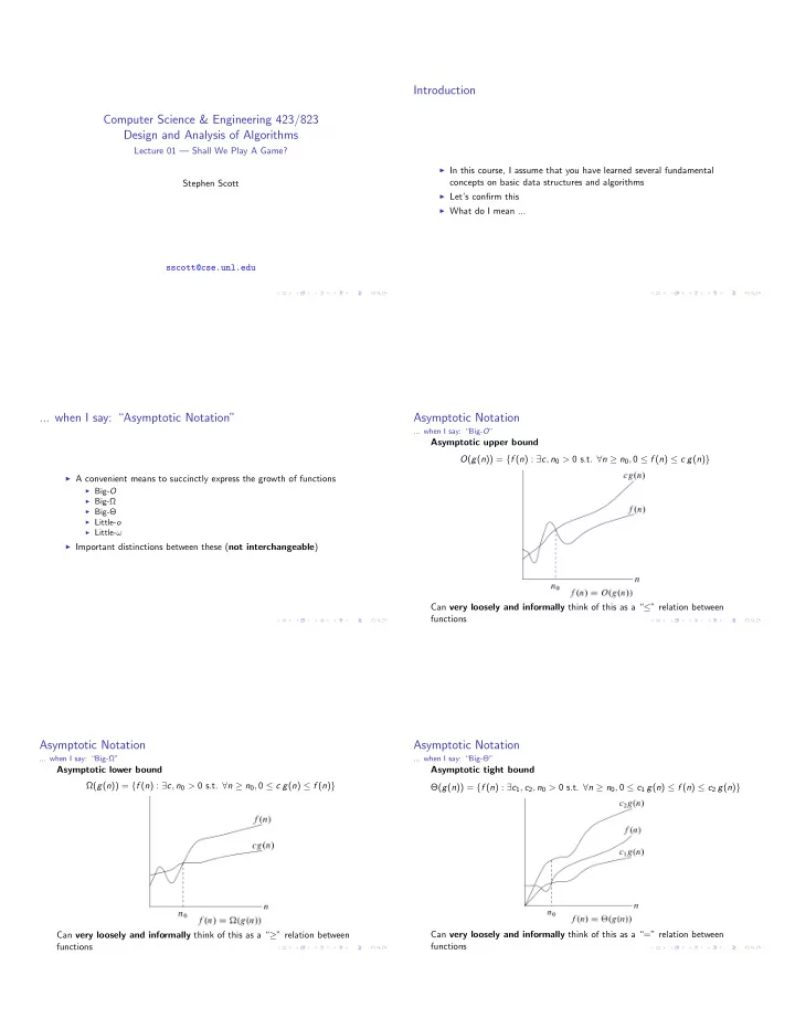
Introduction Computer Science & Engineering 423/823 Design and Analysis of Algorithms Lecture 01 — Shall We Play A Game? I In this course, I assume that you have learned several fundamental concepts on basic data structures and algorithms Stephen Scott I Let’s confirm this I What do I mean ... sscott@cse.unl.edu ... when I say: “Asymptotic Notation” Asymptotic Notation ... when I say: “Big- O ” Asymptotic upper bound O ( g ( n )) = { f ( n ) : 9 c , n 0 > 0 s.t. 8 n � n 0 , 0  f ( n )  c g ( n ) } I A convenient means to succinctly express the growth of functions I Big- O I Big- Ω I Big- Θ I Little- o I Little- ! I Important distinctions between these ( not interchangeable ) Can very loosely and informally think of this as a “  ” relation between functions Asymptotic Notation Asymptotic Notation ... when I say: “Big- Ω ” ... when I say: “Big- Θ ” Asymptotic lower bound Asymptotic tight bound Ω ( g ( n )) = { f ( n ) : 9 c , n 0 > 0 s.t. 8 n � n 0 , 0  c g ( n )  f ( n ) } Θ ( g ( n )) = { f ( n ) : 9 c 1 , c 2 , n 0 > 0 s.t. 8 n � n 0 , 0  c 1 g ( n )  f ( n )  c 2 g ( n ) } Can very loosely and informally think of this as a “ � ” relation between Can very loosely and informally think of this as a “=” relation between functions functions

Asymptotic Notation Asymptotic Notation ... when I say: “Little- o ” ... when I say: “Little- ω ” Upper bound, not asymptotically tight Lower bound, not asymptotically tight o ( g ( n )) = { f ( n ) : 8 c > 0 , 9 n 0 > 0 s.t. 8 n � n 0 , 0  f ( n ) < c g ( n ) } ! ( g ( n )) = { f ( n ) : 8 c > 0 , 9 n 0 > 0 s.t. 8 n � n 0 , 0  c g ( n ) < f ( n ) } Upper inequality strict, and holds for all c > 0 f ( n ) 2 ! ( g ( n )) , g ( n ) 2 o ( f ( n )) Can very loosely and informally think of this as a “ < ” relation between Can very loosely and informally think of this as a “ > ” relation between functions functions ... when I say: “Upper and Lower Bounds” Upper and Lower Bounds ... when I say: “Upper Bound of an Algorithm” I The most common form of analysis I Most often, we analyze algorithms and problems in terms of time I An algorithm A has an upper bound of f ( n ) for input of size n if there complexity (number of operations) exists no input of size n such that A requires more than f ( n ) time I Sometimes we analyze in terms of space complexity (amount of I E.g., we know from prior courses that Quicksort and Bubblesort take no memory) more time than O ( n 2 ), while Mergesort has an upper bound of I Can think of upper and lower bounds of time/space for a specific O ( n log n ) algorithm or a general problem I (But why is Quicksort used more in practice?) I Aside: An algorithm’s lower bound (not typically as interesting) is like a best-case result Upper and Lower Bounds Upper and Lower Bounds ... when I say: “Upper Bound of a Problem” ... when I say: “Lower Bound of a Problem” I A problem has a lower bound of f ( n ) if, for any algorithm A to solve the problem, there exists at least one input of size n that forces A to I A problem has an upper bound of f ( n ) if there exists at least one take at least f ( n ) time/space algorithm that has an upper bound of f ( n ) I This pathological input depends on the specific algorithm A I I.e., there exists an algorithm with time/space complexity of at most f ( n ) I E.g., there is an input of size n (reverse order) that forces Bubblesort to on all inputs of size n take Ω ( n 2 ) steps I E.g., since Mergesort has worst-case time complexity of O ( n log n ), the I Also e.g., there is a di ff erent input of size n that forces Mergesort to problem of sorting has an upper bound of O ( n log n ) I Sorting also has an upper bound of O ( n 2 ) thanks to Bubblesort and take Ω ( n log n ) steps, but none exists forcing ! ( n log n ) steps Quicksort, but this is subsumed by the tighter bound of O ( n log n ) I Since every sorting algorithm has an input of size n forcing Ω ( n log n ) steps, the sorting problem has a time complexity lower bound of Ω ( n log n ) ) Mergesort is asymptotically optimal

Upper and Lower Bounds ... when I say: “E ffi ciency” ... when I say: “Lower Bound of a Problem” (2) I We say that an algorithm is time- or space-e ffi cient if its worst-case time (space) complexity is O ( n c ) for constant c for input size n I To argue a lower bound for a problem, can use an adversarial argument: I I.e., polynomial in the size of the input An algorithm that simulates arbitrary algorithm A to build a I Note on input size: We measure the size of the input in terms of the pathological input number of bits needed to represent it I Needs to be in some general (algorithmic) form since the nature of the I E.g., a graph of n nodes takes O ( n log n ) bits to represent the nodes and O ( n 2 log n ) bits to represent the edges pathological input depends on the specific algorithm A I Can also reduce one problem to another to establish lower bounds I Thus, an algorithm that runs in time O ( n c ) is e ffi cient I In contrast, a problem that includes as an input a numeric parameter k I Spoiler Alert: This semester we will show that if we can compute convex (e.g., threshold) only needs O (log k ) bits to represent hull in o ( n log n ) time, then we can also sort in time o ( n log n ); this I In this case, an e ffi cient algorithm for this problem must run in time cannot be true, so convex hull takes time Ω ( n log n ) O (log c k ) I If instead polynomial in k , sometimes call this pseudopolynomial ... when I say: “Recurrence Relations” Recurrence Relations ... when I say: “Master Theorem” or “Master Method” I We know how to analyze non-recursive algorithms to get asymptotic bounds on run time, but what about recursive ones like Mergesort and Quicksort? I Theorem: Let a � 1 and b > 1 be constants, let f ( n ) be a function, I We use a recurrence relation to capture the time complexity and then and let T ( n ) be defined as T ( n ) = aT ( n / b ) + f ( n ) . Then T ( n ) is bounded as follows: bound the relation asymptotically 1. If f ( n ) = O ( n log b a � ✏ ) for constant ✏ > 0, then T ( n ) = Θ ( n log b a ) I E.g., Mergesort splits the input array of size n into two sub-arrays, 2. If f ( n ) = Θ ( n log b a ), then T ( n ) = Θ ( n log b a log n ) recursively sorts each, and then merges the two sorted lists into a single, 3. If f ( n ) = Ω ( n log b a + ✏ ) for constant ✏ > 0, and if af ( n / b )  cf ( n ) for sorted one constant c < 1 and su ffi ciently large n , then T ( n ) = Θ ( f ( n )) I If T ( n ) is time for Mergesort on n elements, I E.g., for Mergesort, can apply theorem with a = b = 2, use case 2, and n log 2 2 log n � � get T ( n ) = Θ = Θ ( n log n ) T ( n ) = 2 T ( n / 2) + O ( n ) I Still need to get an asymptotic bound on T ( n ) Recurrence Relations Recurrence Relations Other Approaches Still Other Approaches Theorem: For recurrences of the form T ( ↵ n ) + T ( � n ) + O ( n ) for ↵ + � < 1, Previous theorem special case of recursion-tree method : (e.g., T ( n ) = 3 T ( n / 4) + O ( n 2 )) T ( n ) = O ( n ) Proof: Top T ( n ) takes O ( n ) time (= cn for some constant c ). Then calls to T ( ↵ n ) and T ( � n ), which take a total of ( ↵ + � ) cn time, and so on Summing these infinitely yields (since ↵ + � < 1) cn cn (1 + ( ↵ + � ) + ( ↵ + � ) 2 + · · · ) = 1 � ( ↵ + � ) = c 0 n = O ( n ) Another approach is substitution method (guess and prove via induction)

Graphs Graphs ... when I say: “(Undirected) Graph” ... when I say: “Directed Graph” A directed graph (digraph) G = ( V , E ) consists of V , a nonempty set of vertices and E a set of ordered pairs of distinct vertices called edges A (simple, or undirected) graph G = ( V , E ) consists of V , a nonempty set of vertices and E a set of unordered pairs of distinct vertices called edges D E V={A,B,C,D,E} E={ (A,D),(A,E),(B,D), (B,E),(C,D),(C,E)} B A C Graphs Graphs ... when I say: “Weighted Graph” ... when I say: “Representations of Graphs” A weighted graph is an undirected or directed graph with the additional property that each edge e has associated with it a real number w ( e ) called its weight 3 I Two common ways of representing a graph: Adjacency list and adjacency matrix 12 I Let G = ( V , E ) be a graph with n vertices and m edges 0 -6 7 4 3 Graphs Graphs ... when I say: “Adjacency List” ... when I say: “Adjacency Matrix” I Use an n ⇥ n matrix M , where M ( i , j ) = 1 if ( i , j ) is an edge, 0 otherwise I For each vertex v 2 V , store a list of vertices adjacent to v I If G weighted, store weights in the matrix, using 1 for non-edges I For weighted graphs, add information to each node I How much is space required for storage? I How much is space required for storage? a b a b a b c d a a b c d e 0 1 1 1 0 b a e b 1 0 0 0 1 c c c a d c c 1 0 0 1 1 d a c e d 1 0 1 0 1 e b c d d e e 0 1 1 1 0 d e