
1/24
Computer Science & Engineering 423/823 Design and Analysis of Algorithms
Lecture 05 — Elementary Graph Algorithms (Chapter 22) Stephen Scott and Vinodchandran N. Variyam sscott@cse.unl.edu
2/24
Introduction
I Graphs are abstract data types that are applicable to numerous problems
I Can capture entities, relationships between them, the degree of the
relationship, etc.
I This chapter covers basics in graph theory, including representation, and
algorithms for basic graph-theoretic problems (some content was covered in review lecture)
I We’ll build on these later this semester
3/24
Breadth-First Search (BFS)
I Given a graph G = (V , E) (directed or undirected) and a source node
s ∈ V , BFS systematically visits every vertex that is reachable from s
I Uses a queue data structure to search in a breadth-first manner I Creates a structure called a BFS tree such that for each vertex v ∈ V ,
the distance (number of edges) from s to v in tree is a shortest path in G
I Initialize each node’s color to white I As a node is visited, color it to gray (⇒ in queue), then black (⇒
finished)
4/24
BFS(G, s)
1 for each vertex u 2 V \ {s} do 2 color[u] = white 3 d[u] = 1 4 π[u] = nil 5 end 6 color[s] = gray 7 d[s] = 0 8 π[s] = nil 9 Q = ; 10 Enqueue(Q, s) 11 while Q 6= ; do 12 u = Dequeue(Q) 13 for each v 2 Adj[u] do 14 if color[v] == white then 15 color[v] = gray 16 d[v] = d[u] + 1 17 π[v] = u 18 Enqueue(Q, v) 19 20 end 21 color[u] = black 22 end 5/24
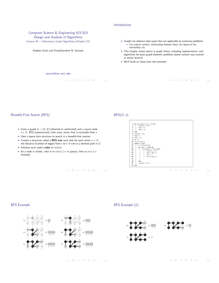
BFS Example
6/24
BFS Example (2)