Introduction CSCE423/823 CSCE423/823 Computer Science & - - PDF document

SLIDE 1 CSCE423/823 Introduction Activity Selection Greedy vs Dynamic Programming Huffman Coding

Computer Science & Engineering 423/823 Design and Analysis of Algorithms

Lecture 10 — Greedy Algorithms (Chapter 16) Stephen Scott (Adapted from Vinodchandran N. Variyam) Spring 2010

1 / 24 CSCE423/823 Introduction Activity Selection Greedy vs Dynamic Programming Huffman Coding

Introduction

Greedy methods: Another optimization technique Similar to dynamic programming in that we examine subproblems, exploiting optimial substructure property Key difference: In dynamic programming we considered all possible subproblems In contrast, a greedy algorithm at each step commits to just one subproblem, which results in its greedy choice (locally optimal choice) Examples: Minimum spanning tree, single-source shortest paths

2 / 24 CSCE423/823 Introduction Activity Selection Optimal Substructure Recursive Definition Greedy Choice Recursive Algorithm Iterative Algorithm Greedy vs Dynamic Programming Huffman Coding

Activity Selection

Consider the problem of scheduling classes in a classroom Many courses are candidates to be scheduled in that room, but not all can have it (can’t hold two courses at once) Want to maximize utilization of the room This is an example of the activity selection problem:

Given: Set S = {a1, a2, . . . , an} of n proposed activities that wish to use a resource that can serve only one activity at a time ai has a start time si and a finish time fi, 0 ≤ si < fi < ∞ If ai is scheduled to use the resource, it occupies it during the interval [si, fi) ⇒ can schedule both ai and aj iff si ≥ fj or sj ≥ fi (if this happens, then we say that ai and aj are compatible) Goal is to find a largest subset S′ ⊆ S such that all activities in S′ are pairwise compatible Assume that activities are sorted by finish time: f1 ≤ f2 ≤ · · · ≤ fn

3 / 24 CSCE423/823 Introduction Activity Selection Optimal Substructure Recursive Definition Greedy Choice Recursive Algorithm Iterative Algorithm Greedy vs Dynamic Programming Huffman Coding

Activity Selection (2)

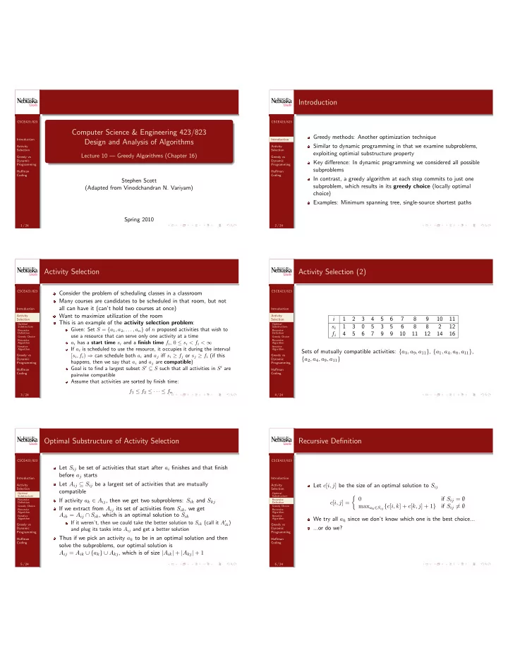
i 1 2 3 4 5 6 7 8 9 10 11 si 1 3 5 3 5 6 8 8 2 12 fi 4 5 6 7 9 9 10 11 12 14 16 Sets of mutually compatible activities: {a3, a9, a11}, {a1, a4, a8, a11}, {a2, a4, a9, a11}

4 / 24 CSCE423/823 Introduction Activity Selection Optimal Substructure Recursive Definition Greedy Choice Recursive Algorithm Iterative Algorithm Greedy vs Dynamic Programming Huffman Coding

Optimal Substructure of Activity Selection

Let Sij be set of activities that start after ai finishes and that finish before aj starts Let Aij ⊆ Sij be a largest set of activities that are mutually compatible If activity ak ∈ Aij, then we get two subproblems: Sik and Skj If we extract from Aij its set of activities from Sik, we get Aik = Aij ∩ Sik, which is an optimal solution to Sik

If it weren’t, then we could take the better solution to Sik (call it A′

ik)

and plug its tasks into Aij and get a better solution

Thus if we pick an activity ak to be in an optimal solution and then solve the subproblems, our optimal solution is Aij = Aik ∪ {ak} ∪ Akj, which is of size |Aik| + |Akj| + 1

5 / 24 CSCE423/823 Introduction Activity Selection Optimal Substructure Recursive Definition Greedy Choice Recursive Algorithm Iterative Algorithm Greedy vs Dynamic Programming Huffman Coding

Recursive Definition

Let c[i, j] be the size of an optimal solution to Sij c[i, j] = if Sij = ∅ maxak∈Sij{c[i, k] + c[k, j] + 1} if Sij = ∅ We try all ak since we don’t know which one is the best choice... ...or do we?

6 / 24

SLIDE 2 CSCE423/823 Introduction Activity Selection Optimal Substructure Recursive Definition Greedy Choice Recursive Algorithm Iterative Algorithm Greedy vs Dynamic Programming Huffman Coding

Greedy Choice

What if, instead of trying all activities ak, we simply chose the one with the earliest finish time of all those still compatible with the scheduled ones? This is a greedy choice in that it maximizes the amount of time left

• ver to schedule other activities

Let Sk = {ai ∈ S : si ≥ fk} be set of activities that start after ak finishes If we greedily choose a1 first (with earliest finish time), then S1 is the only subproblem to solve

7 / 24 CSCE423/823 Introduction Activity Selection Optimal Substructure Recursive Definition Greedy Choice Recursive Algorithm Iterative Algorithm Greedy vs Dynamic Programming Huffman Coding

Greedy Choice (2)

Theorem: Consider any nonempty subproblem Sk and let am be an activity in Sk with earliest finish time. Then am is in some maximum-size subset of mutually compatible activities of Sk

Let Ak be an optimal solution to Sk and let aj have earliest finish time of all in Ak If aj = am, we’re done If aj = am, then define A′

k = Ak \ {aj} ∪ {am}

Activities in A′ are mutually compatible since those in A are mutually compatible and fm ≤ fj Since |A′

k| = |Ak|, we get that A′ k is a maximum-size subset of

mutually compatible activities of Sk that includes am

What this means is that there is an optimal solution that uses the greedy choice

8 / 24 CSCE423/823 Introduction Activity Selection Optimal Substructure Recursive Definition Greedy Choice Recursive Algorithm Iterative Algorithm Greedy vs Dynamic Programming Huffman Coding

Recursive Algorithm

m = k + 1

1

while m ≤ n and s[m] < f[k] do

2

m = m + 1

3

end

4

if m ≤ n then

5

return {am}∪ Recursive-Activity-

6

Selector(s, f, m, n) else return ∅

7

Algorithm 1: Recursive-Activity- Selector(s, f, k, n)

9 / 24 CSCE423/823 Introduction Activity Selection Optimal Substructure Recursive Definition Greedy Choice Recursive Algorithm Iterative Algorithm Greedy vs Dynamic Programming Huffman Coding

Recursive Algorithm (2)

10 / 24 CSCE423/823 Introduction Activity Selection Optimal Substructure Recursive Definition Greedy Choice Recursive Algorithm Iterative Algorithm Greedy vs Dynamic Programming Huffman Coding

Iterative Algorithm

A = {a1}

1

k = 1

2

for m = 2 to n do

3

if s[m] ≥ f[k] then

4

A = A ∪ {am}

5

k = m

6

end

7

return A

8

Algorithm 2: Greedy-Activity-Selector(s, f, n) What is the time complexity? What would it have been if we’d approached this as a DP problem?

11 / 24 CSCE423/823 Introduction Activity Selection Greedy vs Dynamic Programming Huffman Coding

Greedy vs Dynamic Programming

When can we get away with a greedy algorithm instead of DP? When we can argue that the greedy choice is part of an optimal solution, implying that we need not explore all subproblems Example: The knapsack problem

There are n items that a thief can steal, item i weighing wi pounds and worth vi dollars The thief’s goal is to steal a set of items weighing at most W pounds and maximizes total value In the 0-1 knapsack problem, each item must be taken in its entirety (e.g. gold bars) In the fractional knapsack problem, the thief can take part of an item and get a proportional amount of its value (e.g. gold dust)

12 / 24

SLIDE 3 CSCE423/823 Introduction Activity Selection Greedy vs Dynamic Programming Huffman Coding

Greedy vs Dynamic Programming (2)

There’s a greedy algorithm for the fractional knapsack problem

Sort the items by vi/wi and choose the items in descending order Has greedy choice property, since any optimal solution lacking the greedy choice can have the greedy choice swapped in

Works because one can always completely fill the knapsack at the last step

Greedy strategy does not work for 0-1 knapsack, but do have O(nW)-time dynamic programming algorithm

Note that time complexity is pseudopolynomial Decision problem is NP-complete

13 / 24 CSCE423/823 Introduction Activity Selection Greedy vs Dynamic Programming Huffman Coding

Greedy vs Dynamic Programming (3)

Problem instance 0-1 (greedy is suboptimal) Fractional

14 / 24 CSCE423/823 Introduction Activity Selection Greedy vs Dynamic Programming Huffman Coding Algorihtm Greedy Choice Property Optimal Substructure Property

Huffman Coding

Interested in encoding a file of symbols from some alphabet Want to minimize the size of the file, based on the frequencies of the symbols A fixed-length code uses ⌈log2 n⌉ bits per symbol, where n is the size of the alphabet C A variable-length code uses fewer bits for more frequent symbols a b c d e f Frequency (in thousands) 45 13 12 16 9 5 Fixed-length codeword 000 001 010 011 100 101 Variable-length codeword 101 100 111 1101 1100 Fixed-length code uses 300k bits, variable-length uses 224k bits

15 / 24 CSCE423/823 Introduction Activity Selection Greedy vs Dynamic Programming Huffman Coding Algorihtm Greedy Choice Property Optimal Substructure Property

Huffman Coding (2)

Can represent any encoding as a binary tree If c.freq = frequency of codeword and dT (c) = depth, cost of tree T is B(T) =

• c∈C

c.freq · dT (c)

16 / 24 CSCE423/823 Introduction Activity Selection Greedy vs Dynamic Programming Huffman Coding Algorihtm Greedy Choice Property Optimal Substructure Property

Algorihtm for Optimal Codes

Can get an optimal code by finding an appropriate prefix code, where no codeword is a prefix of another Optimal code also corresponds to a full binary tree Huffman’s algorithm builds an optimal code by greedily building its tree Given alphabet C (which corresponds to leaves), find the two least frequent ones, merge them into a subtree Frequency of new subtree is the sum of the frequencies of its children Then add the subtree back into the set for future consideration

17 / 24 CSCE423/823 Introduction Activity Selection Greedy vs Dynamic Programming Huffman Coding Algorihtm Greedy Choice Property Optimal Substructure Property

Algorihtm for Optimal Codes (2)

n = |C|

1

Q = C // min-priority queue

2

for i = 1 to n − 1 do

3

allocate node z

4

z.left = x = Extract-Min(Q)

5

z.right = y = Extract-Min(Q)

6

z.freq = x.freq + y.freq

7

Insert(Q, z)

8

end

9

return Extract-Min(Q) // return root

10

Algorithm 3: Huffman(C)

Time complexity: n − 1 iterations, O(log n) time per iteration, total O(n log n)

18 / 24

SLIDE 4 CSCE423/823 Introduction Activity Selection Greedy vs Dynamic Programming Huffman Coding Algorihtm Greedy Choice Property Optimal Substructure Property

Algorithm for Optimal Codes (3)

19 / 24 CSCE423/823 Introduction Activity Selection Greedy vs Dynamic Programming Huffman Coding Algorihtm Greedy Choice Property Optimal Substructure Property

Optimal Coding Has Greedy Choice Property

Lemma: Let C be an alphabet in which symbol c ∈ C has frequency c.freq and let x, y ∈ C have lowest frequencies. Then there exists an optimal prefix code for C in which codewords for x and y have same length and differ only in the last bit. Proof: Let T be a tree representing an arbitrary optimal prefix code, and let a and b be siblings of maximum depth in T Assume, w.l.o.g., that x.freq ≤ y.freq and a.freq ≤ b.freq Since x and y are the two least frequent nodes, we get x.freq ≤ a.freq and y.freq ≤ b.freq Convert T to T ′ by exchanging a and x, then convert to T ′′ by exchanging b and y In T ′′, x and y are siblings of maximum depth

20 / 24 CSCE423/823 Introduction Activity Selection Greedy vs Dynamic Programming Huffman Coding Algorihtm Greedy Choice Property Optimal Substructure Property

Optimal Coding Has Greedy Choice Property (2)

21 / 24 CSCE423/823 Introduction Activity Selection Greedy vs Dynamic Programming Huffman Coding Algorihtm Greedy Choice Property Optimal Substructure Property

Optimal Coding Has Greedy Choice Property (3)

Cost difference between T and T ′ is B(T) − B(T ′): =

• c∈C

c.freq · dT (c) −

• c∈C

c.freq · dT ′(c) = x.freq · dT (x) + a.freq · dT (a) − x.freq · dT ′(x) − a.freq · dT ′(a) = x.freq · dT (x) + a.freq · dT (a) − x.freq · dT (a) − x.freq · dT (x) = (a.freq − x.freq)(dT (a) − dT (x)) ≥ 0 since a.freq ≥ x.freq and dT (a) ≥ dT (x) Similarly, B(T ′) − B(T ′′) ≥ 0, so B(T ′′) ≤ B(T), so T ′′ is optimal

22 / 24 CSCE423/823 Introduction Activity Selection Greedy vs Dynamic Programming Huffman Coding Algorihtm Greedy Choice Property Optimal Substructure Property

Optimal Coding Has Optimal Substructure Property

Lemma: Let C be an alphabet in which symbol c ∈ C has frequency c.freq and let x, y ∈ C have lowest frequencies. Let C′ = C \ {x, y} ∪ {z} and z.freq = x.freq + y.freq. Let T ′ be any tree representing an optimal prefix code for C′. Then T, which is T ′ with leaf z replaced by internal node with children x and y, represents an optimal prefix code for C Proof: Since dT (x) = dT (y) = dT ′(z) + 1, x.freq · dT (x) + y.freq · dT (y) = (x.freq + y.freq)(dT ′(z) + 1) = z.freq · dT ′(z) + (x.freq + y.freq) Also, since dT (c) = dT ′(c) for all c ∈ C \ {x, y}, B(T) = B(T ′) + x.freq + y.freq and B(T ′) = B(T) − x.freq − y.freq

23 / 24 CSCE423/823 Introduction Activity Selection Greedy vs Dynamic Programming Huffman Coding Algorihtm Greedy Choice Property Optimal Substructure Property

Optimal Coding Has Optimal Substructure Property (2)

Assume that T is not optimal, i.e. B(T ′′) < B(T) for some T ′′ Assume w.l.o.g. (based on previous lemma) that x and y are siblings in T ′′ In T ′′, replace x, y, and their parent with z such that z.freq = x.freq + y.freq, to get T ′′′:

B(T ′′′) = B(T ′′) − x.freq − y.freq (from prev. slide) < B(T) − x.freq − y.freq (from T suboptimal assumption) = B(T ′) (from prev. slide)

This contradicts assumption that T ′ is optimal for C′

24 / 24