Introduction CSCE423/823 CSCE423/823 Computer Science & - - PDF document

SLIDE 1 CSCE423/823 Introduction Rod Cutting Matrix-Chain Multiplication Longest Common Subsequence Optimal Binary Search Trees

Computer Science & Engineering 423/823 Design and Analysis of Algorithms

Lecture 09 — Dynamic Programming (Chapter 15) Stephen Scott (Adapted from Vinodchandran N. Variyam)

1 / 42 CSCE423/823 Introduction Rod Cutting Matrix-Chain Multiplication Longest Common Subsequence Optimal Binary Search Trees

Introduction

Dynamic programming is a technique for solving optimization problems Key element: Decompose a problem into subproblems, solve them recursively, and then combine the solutions into a final (optimal) solution Important component: There are typically an exponential number of subproblems to solve, but many of them overlap ) Can re-use the solutions rather than re-solving them Number of distinct subproblems is polynomial

2 / 42 CSCE423/823 Introduction Rod Cutting Recursive Algorithm Dynamic Programming Algorithm Reconstructing a Solution Matrix-Chain Multiplication Longest Common Subsequence Optimal Binary Search Trees

Rod Cutting

A company has a rod of length n and wants to cut it into smaller rods to maximize profit Have a table telling how much they get for rods of various lengths: A rod of length i has price pi The cuts themselves are free, so profit is based solely on the prices charged for of the rods If cuts only occur at integral boundaries 1, 2, . . . , n 1, then can make or not make a cut at each of n 1 positions, so total number

• f possible solutions is 2n1

3 / 42 CSCE423/823 Introduction Rod Cutting Recursive Algorithm Dynamic Programming Algorithm Reconstructing a Solution Matrix-Chain Multiplication Longest Common Subsequence Optimal Binary Search Trees

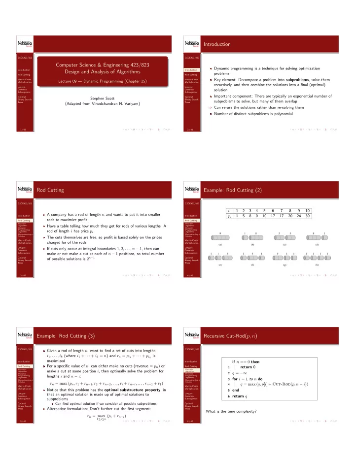
Example: Rod Cutting (2)

i 1 2 3 4 5 6 7 8 9 10 pi 1 5 8 9 10 17 17 20 24 30

4 / 42 CSCE423/823 Introduction Rod Cutting Recursive Algorithm Dynamic Programming Algorithm Reconstructing a Solution Matrix-Chain Multiplication Longest Common Subsequence Optimal Binary Search Trees

Example: Rod Cutting (3)

Given a rod of length n, want to find a set of cuts into lengths i1, . . . , ik (where i1 + · · · + ik = n) and rn = pi1 + · · · + pik is maximized For a specific value of n, can either make no cuts (revenue = pn) or make a cut at some position i, then optimally solve the problem for lengths i and n i: rn = max (pn, r1 + rn1, r2 + rn2, . . . , ri + rni, . . . , rn1 + r1) Notice that this problem has the optimal substructure property, in that an optimal solution is made up of optimal solutions to subproblems

Can find optimal solution if we consider all possible subproblems

Alternative formulation: Don’t further cut the first segment: rn = max

1in (pi + rni)

5 / 42 CSCE423/823 Introduction Rod Cutting Recursive Algorithm Dynamic Programming Algorithm Reconstructing a Solution Matrix-Chain Multiplication Longest Common Subsequence Optimal Binary Search Trees

Recursive Cut-Rod(p, n)

if n == 0 then

1

return 0

2 q = 1 3 for i = 1 to n do 4

q = max (q, p[i] + Cut-Rod(p, n i))

5 end 6 return q

What is the time complexity?

6 / 42

SLIDE 2 CSCE423/823 Introduction Rod Cutting Recursive Algorithm Dynamic Programming Algorithm Reconstructing a Solution Matrix-Chain Multiplication Longest Common Subsequence Optimal Binary Search Trees

Time Complexity

Let T(n) be number of calls to Cut-Rod Thus T(0) = 1 and, based on the for loop, T(n) = 1 +

n1

X

j=0

T(j) = 2n Why exponential? Cut-Rod exploits the optimal substructure property, but repeats work on these subproblems E.g. if the first call is for n = 4, then there will be:

1 call to Cut-Rod(4) 1 call to Cut-Rod(3) 2 calls to Cut-Rod(2) 4 calls to Cut-Rod(1) 8 calls to Cut-Rod(0)

7 / 42 CSCE423/823 Introduction Rod Cutting Recursive Algorithm Dynamic Programming Algorithm Reconstructing a Solution Matrix-Chain Multiplication Longest Common Subsequence Optimal Binary Search Trees

Time Complexity (2)

Recursion Tree for n = 4

8 / 42 CSCE423/823 Introduction Rod Cutting Recursive Algorithm Dynamic Programming Algorithm Reconstructing a Solution Matrix-Chain Multiplication Longest Common Subsequence Optimal Binary Search Trees

Dynamic Programming Algorithm

Can save time dramatically by remembering results from prior calls Two general approaches:

1

Top-down with memoization: Run the recursive algorithm as defined earlier, but before recursive call, check to see if the calculation has already been done and memoized

2

Bottom-up: Fill in results for “small” subproblems first, then use these to fill in table for “larger” ones

Typically have the same asymptotic running time

9 / 42 CSCE423/823 Introduction Rod Cutting Recursive Algorithm Dynamic Programming Algorithm Reconstructing a Solution Matrix-Chain Multiplication Longest Common Subsequence Optimal Binary Search Trees

Memoized-Cut-Rod-Aux(p, n, r)

if r[n] 0 then

1

return r[n] // r initialized to all 1

2

if n == 0 then

3

q = 0

4

else

5

q = 1

6

for i = 1 to n do

7

q = max (q, p[i] + Memoized-Cut-Rod-Aux(p, n i, r))

8

end

9

r[n] = q

10

return q

10 / 42 CSCE423/823 Introduction Rod Cutting Recursive Algorithm Dynamic Programming Algorithm Reconstructing a Solution Matrix-Chain Multiplication Longest Common Subsequence Optimal Binary Search Trees

Bottom-Up-Cut-Rod(p, n)

Allocate r[0 . . . n]

1

r[0] = 0

2

for j = 1 to n do

3

q = 1

4

for i = 1 to j do

5

q = max (q, p[i] + r[j i])

6

end

7

r[j] = q

8

end

9

return r[n]

First solves for n = 0, then for n = 1 in terms of r[0], then for n = 2 in terms of r[0] and r[1], etc.

11 / 42 CSCE423/823 Introduction Rod Cutting Recursive Algorithm Dynamic Programming Algorithm Reconstructing a Solution Matrix-Chain Multiplication Longest Common Subsequence Optimal Binary Search Trees

Time Complexity

Subproblem graph for n = 4 Both algorithms take linear time to solve for each value of n, so total time complexity is Θ(n2)

12 / 42

SLIDE 3 CSCE423/823 Introduction Rod Cutting Recursive Algorithm Dynamic Programming Algorithm Reconstructing a Solution Matrix-Chain Multiplication Longest Common Subsequence Optimal Binary Search Trees

Reconstructing a Solution

If interested in the set of cuts for an optimal solution as well as the revenue it generates, just keep track of the choice made to optimize each subproblem Will add a second array s, which keeps track of the optimal size of the first piece cut in each subproblem

13 / 42 CSCE423/823 Introduction Rod Cutting Recursive Algorithm Dynamic Programming Algorithm Reconstructing a Solution Matrix-Chain Multiplication Longest Common Subsequence Optimal Binary Search Trees

Extended-Bottom-Up-Cut-Rod(p, n)

Allocate r[0 . . . n] and s[0 . . . n]

1

r[0] = 0

2

for j = 1 to n do

3

q = 1

4

for i = 1 to j do

5

if q < p[i] + r[j i] then

6

q = p[i] + r[j i]

7

s[j] = i

8 9

end

10

r[j] = q

11

end

12

return r, s

14 / 42 CSCE423/823 Introduction Rod Cutting Recursive Algorithm Dynamic Programming Algorithm Reconstructing a Solution Matrix-Chain Multiplication Longest Common Subsequence Optimal Binary Search Trees

Print-Cut-Rod-Solution(p, n)

(r, s) = Extended-Bottom-Up-Cut-Rod(p, n)

1

while n > 0 do

2

print s[n]

3

n = n s[n]

4

end

Example: i 1 2 3 4 5 6 7 8 9 10 r[i] 1 5 8 10 13 17 18 22 25 30 s[i] 1 2 3 2 2 6 1 2 3 10 If n = 10, optimal solution is no cut; if n = 7, then cut once to get segments of sizes 1 and 6

15 / 42 CSCE423/823 Introduction Rod Cutting Matrix-Chain Multiplication Characterizing Structure Recursive Definition Computing Optimal Value Constructing Optimal Solution Overalapping Subproblems Longest Common Subsequence Optimal Binary Search Trees

Matrix-Chain Multiplication

Given a chain of matrices hA1, . . . , Ani, goal is to compute their product A1 · · · An This operation is associative, so can sequence the multiplications in multiple ways and get the same result Can cause dramatic changes in number of operations required Multiplying a p ⇥ q matrix by a q ⇥ r matrix requires pqr steps and yields a p ⇥ r matrix for future multiplications E.g. Let A1 be 10 ⇥ 100, A2 be 100 ⇥ 5, and A3 be 5 ⇥ 50

1

Computing ((A1A2)A3) requires 10 · 100 · 5 = 5000 steps to compute (A1A2) (yielding a 10 ⇥ 5), and then 10 · 5 · 50 = 2500 steps to finish, for a total of 7500

2

Computing (A1(A2A3)) requires 100 · 5 · 50 = 25000 steps to compute (A2A3) (yielding a 100 ⇥ 50), and then 10 · 100 · 50 = 50000 steps to finish, for a total of 75000

16 / 42 CSCE423/823 Introduction Rod Cutting Matrix-Chain Multiplication Characterizing Structure Recursive Definition Computing Optimal Value Constructing Optimal Solution Overalapping Subproblems Longest Common Subsequence Optimal Binary Search Trees

Matrix-Chain Multiplication (2)

The matrix-chain multiplication problem is to take a chain hA1, . . . , Ani of n matrices, where matrix i has dimension pi1 ⇥ pi, and fully parenthesize the product A1 · · · An so that the number of scalar multiplications is minimized Brute force solution is infeasible, since its time complexity is Ω

• 4n/n3/2

Will follow 4-step procedure for dynamic programming:

1

Characterize the structure of an optimal solution

2

Recursively define the value of an optimal solution

3

Compute the value of an optimal solution

4

Construct an optimal solution from computed information

17 / 42 CSCE423/823 Introduction Rod Cutting Matrix-Chain Multiplication Characterizing Structure Recursive Definition Computing Optimal Value Constructing Optimal Solution Overalapping Subproblems Longest Common Subsequence Optimal Binary Search Trees

Characterizing the Structure of an Optimal Solution

Let Ai...j be the matrix from the product AiAi+1 · · · Aj To compute Ai...j, must split the product and compute Ai...k and Ak+1...j for some integer k, then multiply the two together Cost is the cost of computing each subproduct plus cost of multiplying the two results Say that in an optimal parenthesization, the optimal split for AiAi+1 · · · Aj is at k Then in an optimal solution for AiAi+1 · · · Aj, the parenthisization of Ai · · · Ak is itself optimal for the subchain Ai · · · Ak (if not, then we could do better for the larger chain) Similar argument for Ak+1 · · · Aj Thus if we make the right choice for k and then optimally solve the subproblems recursively, we’ll end up with an optimal solution Since we don’t know optimal k, we’ll try them all

18 / 42

SLIDE 4 CSCE423/823 Introduction Rod Cutting Matrix-Chain Multiplication Characterizing Structure Recursive Definition Computing Optimal Value Constructing Optimal Solution Overalapping Subproblems Longest Common Subsequence Optimal Binary Search Trees

Recursively Defining the Value of an Optimal Solution

Define m[i, j] as minimum number of scalar multiplications needed to compute Ai...j (What entry in the m table will be our final answer?) Computing m[i, j]:

1

If i = j, then no operations needed and m[i, i] = 0 for all i

2

If i < j and we split at k, then optimal number of operations needed is the optimal number for computing Ai...k and Ak+1...j, plus the number to multiply them: m[i, j] = m[i, k] + m[k + 1, j] + pi1pkpj

3

Since we don’t know k, we’ll try all possible values: m[i, j] = ⇢ 0 if i = j minik<j{m[i, k] + m[k + 1, j] + pi1pkpj} if i < j

To track the optimal solution itself, define s[i, j] to be the value of k used at each split

19 / 42 CSCE423/823 Introduction Rod Cutting Matrix-Chain Multiplication Characterizing Structure Recursive Definition Computing Optimal Value Constructing Optimal Solution Overalapping Subproblems Longest Common Subsequence Optimal Binary Search Trees

Computing the Value of an Optimal Solution

As with the rod cutting problem, many of the subproblems we’ve defined will overlap Exploiting overlap allows us to solve only Θ(n2) problems (one problem for each (i, j) pair), as opposed to exponential We’ll do a bottom-up implementation, based on chain length Chains of length 1 are trivially solved (m[i, i] = 0 for all i) Then solve chains of length 2, 3, etc., up to length n Linear time to solve each problem, quadratic number of problems, yields O(n3) total time

20 / 42 CSCE423/823 Introduction Rod Cutting Matrix-Chain Multiplication Characterizing Structure Recursive Definition Computing Optimal Value Constructing Optimal Solution Overalapping Subproblems Longest Common Subsequence Optimal Binary Search Trees

Matrix-Chain-Order(p, n)

allocate m[1 . . . n, 1 . . . n] and s[1 . . . n, 1 . . . n] 1 initialize m[i, i] = 0 8 1  i  n 2 for ` = 2 to n do 3 for i = 1 to n ` + 1 do 4 j = i + ` 1 5 m[i, j] = 1 6 for k = i to j 1 do 7 q = m[i, k] + m[k + 1, j] + pi−1pkpj 8 if q < m[i, j] then 9 m[i, j] = q 10 s[i, j] = k 11 12 end 13 end 14 end 15 return (m, s) 21 / 42 CSCE423/823 Introduction Rod Cutting Matrix-Chain Multiplication Characterizing Structure Recursive Definition Computing Optimal Value Constructing Optimal Solution Overalapping Subproblems Longest Common Subsequence Optimal Binary Search Trees

Computing the Value of an Optimal Solution (3)

matrix A1 A2 A3 A4 A5 A6 dimension 30 ⇥ 35 35 ⇥ 15 15 ⇥ 5 5 ⇥ 10 10 ⇥ 20 20 ⇥ 25

22 / 42 CSCE423/823 Introduction Rod Cutting Matrix-Chain Multiplication Characterizing Structure Recursive Definition Computing Optimal Value Constructing Optimal Solution Overalapping Subproblems Longest Common Subsequence Optimal Binary Search Trees

Constructing an Optimal Solution from Computed Information

Cost of optimal parenthesization is stored in m[1, n] First split in optimal parenthesization is between s[1, n] and s[1, n] + 1 Descending recursively, next splits are between s[1, s[1, n]] and s[1, s[1, n]] + 1 for left side and between s[s[1, n] + 1, n] and s[s[1, n] + 1, n] + 1 for right side and so on...

23 / 42 CSCE423/823 Introduction Rod Cutting Matrix-Chain Multiplication Characterizing Structure Recursive Definition Computing Optimal Value Constructing Optimal Solution Overalapping Subproblems Longest Common Subsequence Optimal Binary Search Trees

Print-Optimal-Parens(s, i, j)

if i == j then

1

print “A”i

2 else 3

print “(”

4

Print-Optimal-Parens(s, i, s[i, j])

5

Print-Optimal-Parens(s, s[i, j] + 1, j)

6

print “)”

7 24 / 42

SLIDE 5 CSCE423/823 Introduction Rod Cutting Matrix-Chain Multiplication Characterizing Structure Recursive Definition Computing Optimal Value Constructing Optimal Solution Overalapping Subproblems Longest Common Subsequence Optimal Binary Search Trees

Constructing an Optimal Solution from Computed Information (3)

Optimal parenthesization: ((A1(A2A3))((A4A5)A6))

25 / 42 CSCE423/823 Introduction Rod Cutting Matrix-Chain Multiplication Characterizing Structure Recursive Definition Computing Optimal Value Constructing Optimal Solution Overalapping Subproblems Longest Common Subsequence Optimal Binary Search Trees

Example of How Subproblems Overlap

Entire subtrees overlap: See Section 15.3 for more on optimal substructure and overlapping subproblems

26 / 42 CSCE423/823 Introduction Rod Cutting Matrix-Chain Multiplication Longest Common Subsequence Characterizing Structure Recursive Definition Computing Optimal Value Constructing Optimal Solution Optimal Binary Search Trees

Longest Common Subsequence

Sequence Z = hz1, z2, . . . , zki is a subsequence of another sequence X = hx1, x2, . . . , xmi if there is a strictly increasing sequence hi1, . . . , iki of indices of X such that for all j = 1, . . . , k, xij = zj I.e. as one reads through Z, one can find a match to each symbol of Z in X, in order (though not necessarily contiguous) E.g. Z = hB, C, D, Bi is a subsequence of X = hA, B, C, B, D, A, Bi since z1 = x2, z2 = x3, z3 = x5, and z4 = x7 Z is a common subsequence of X and Y if it is a subsequence of both The goal of the longest common subsequence problem is to find a maximum-length common subsequence (LCS) of sequences X = hx1, x2, . . . , xmi and Y = hy1, y2, . . . , yni

27 / 42 CSCE423/823 Introduction Rod Cutting Matrix-Chain Multiplication Longest Common Subsequence Characterizing Structure Recursive Definition Computing Optimal Value Constructing Optimal Solution Optimal Binary Search Trees

Characterizing the Structure of an Optimal Solution

Given sequence X = hx1, . . . , xmi, the ith prefix of X is Xi = hx1, . . . , xii Theorem If X = hx1, . . . , xmi and Y = hy1, . . . , yni have LCS Z = hz1, . . . , zki, then

1

xm = yn ) zk = xm = yn and Zk1 is LCS of Xm1 and Yn1

If zk 6= xm, can lengthen Z, ) contradiction If Zk1 not LCS of Xm1 and Yn1, then a longer CS of Xm1 and Yn1 could have xm appended to it to get CS of X and Y that is longer than Z, ) contradiction

2

If xm 6= yn, then zk 6= xm implies that Z is an LCS of Xm1 and Y

If zk 6= xm, then Z is a CS of Xm1 and Y . Any CS of Xm1 and Y that is longer than Z would also be a longer CS for X and Y , ) contradiction

3

If xm 6= yn, then zk 6= yn implies that Z is an LCS of X and Yn1

Similar argument to (2)

28 / 42 CSCE423/823 Introduction Rod Cutting Matrix-Chain Multiplication Longest Common Subsequence Characterizing Structure Recursive Definition Computing Optimal Value Constructing Optimal Solution Optimal Binary Search Trees

Recursively Defining the Value of an Optimal Solution

The theorem implies the kinds of subproblems that we’ll investigate to find LCS of X = hx1, . . . , xmi and Y = hy1, . . . , yni If xm = yn, then find LCS of Xm1 and Yn1 and append xm (= yn) to it If xm 6= yn, then find LCS of X and Yn1 and find LCS of Xm1 and Y and identify the longest one Let c[i, j] = length of LCS of Xi and Yj c[i, j] = 8 < : if i = 0 or j = 0 c[i 1, j 1] + 1 if i, j > 0 and xi = yj max (c[i, j 1], c[i 1, j]) if i, j > 0 and xi 6= yj

29 / 42 CSCE423/823 Introduction Rod Cutting Matrix-Chain Multiplication Longest Common Subsequence Characterizing Structure Recursive Definition Computing Optimal Value Constructing Optimal Solution Optimal Binary Search Trees

LCS-Length(X, Y, m, n)

allocate b[1 . . . m, 1 . . . n] and c[0 . . . m, 0 . . . n] 1 initialize c[i, 0] = 0 and c[0, j] = 0 8 0  i  m and 0  j  n 2 for i = 1 to m do 3 for j = 1 to n do 4 if xi == yj then 5 c[i, j] = c[i 1, j 1] + 1 6 b[i, j] = “ - ” 7 else if c[i 1, j] c[i, j 1] then 8 c[i, j] = c[i 1, j] 9 b[i, j] = “ " ” 10 else 11 c[i, j] = c[i, j 1] 12 b[i, j] = “ ” 13 14 end 15 end 16 return (c, b)

What is the time complexity?

30 / 42

SLIDE 6 CSCE423/823 Introduction Rod Cutting Matrix-Chain Multiplication Longest Common Subsequence Characterizing Structure Recursive Definition Computing Optimal Value Constructing Optimal Solution Optimal Binary Search Trees

Computing the Value of an Optimal Solution (2)

X = hA, B, C, B, D, A, Bi, Y = hB, D, C, A, B, Ai

31 / 42 CSCE423/823 Introduction Rod Cutting Matrix-Chain Multiplication Longest Common Subsequence Characterizing Structure Recursive Definition Computing Optimal Value Constructing Optimal Solution Optimal Binary Search Trees

Constructing an Optimal Solution from Computed Information

Length of LCS is stored in c[m, n] To print LCS, start at b[m, n] and follow arrows until in row or column 0 If in cell (i, j) on this path, when xi = yj (i.e. when arrow is “ - ”), print xi as part of the LCS This will print LCS backwards

32 / 42 CSCE423/823 Introduction Rod Cutting Matrix-Chain Multiplication Longest Common Subsequence Characterizing Structure Recursive Definition Computing Optimal Value Constructing Optimal Solution Optimal Binary Search Trees

Print-LCS(b, X, i, j)

if i == 0 or j == 0 then

1

return

2 if b[i, j] == “ - ” then 3

Print-LCS(b, X, i 1, j 1)

4

print xi

5 else if b[i, j] == “ " ” then 6

Print-LCS(b, X, i 1, j)

7 else Print-LCS(b, X, i, j 1)

What is the time complexity?

33 / 42 CSCE423/823 Introduction Rod Cutting Matrix-Chain Multiplication Longest Common Subsequence Characterizing Structure Recursive Definition Computing Optimal Value Constructing Optimal Solution Optimal Binary Search Trees

Constructing an Optimal Solution from Computed Information (3)

X = hA, B, C, B, D, A, Bi, Y = hB, D, C, A, B, Ai, prints “BCBA”

34 / 42 CSCE423/823 Introduction Rod Cutting Matrix-Chain Multiplication Longest Common Subsequence Optimal Binary Search Trees Characterizing Structure Recursive Definition Computing Optimal Value Constructing Optimal Solution

Optimal Binary Search Trees

Goal is to construct binary search trees such that most frequently sought values are near the root, thus minimizing expected search time Given a sequence K = hk1, . . . , kni of n distinct keys in sorted order Key ki has probability pi that it will be sought on a particular search To handle searches for values not in K, have n + 1 dummy keys d0, d1, . . . , dn to serve as the tree’s leaves Dummy key di will be reached with probability qi If depthT (ki) is distance from root of ki in tree T, then expected search cost of T is 1 +

n

X

i=1

pi depthT (ki) +

n

X

i=0

qi depthT (di) An optimal binary search tree is one with minimum expected search cost

35 / 42 CSCE423/823 Introduction Rod Cutting Matrix-Chain Multiplication Longest Common Subsequence Optimal Binary Search Trees Characterizing Structure Recursive Definition Computing Optimal Value Constructing Optimal Solution

Optimal Binary Search Trees (2)

i 1 2 3 4 5 pi 0.15 0.10 0.05 0.10 0.20 qi 0.05 0.10 0.05 0.05 0.05 0.10

expected cost = 2.80 expected cost = 2.75 (optimal)

36 / 42

SLIDE 7 CSCE423/823 Introduction Rod Cutting Matrix-Chain Multiplication Longest Common Subsequence Optimal Binary Search Trees Characterizing Structure Recursive Definition Computing Optimal Value Constructing Optimal Solution

Characterizing the Structure of an Optimal Solution

Observation: Since K is sorted and dummy keys interspersed in

• rder, any subtree of a BST must contain keys in a contiguous range

ki, . . . , kj and have leaves di1, . . . , dj Thus, if an optimal BST T has a subtree T 0 over keys ki, . . . , kj, then T 0 is optimal for the subproblem consisting of only the keys ki, . . . , kj

If T 0 weren’t optimal, then a lower-cost subtree could replace T 0 in T, ) contradiction

Given keys ki, . . . , kj, say that its optimal BST roots at kr for some i  r  j Thus if we make right choice for kr and optimally solve the problem for ki, . . . , kr1 (with dummy keys di1, . . . , dr1) and the problem for kr+1, . . . , kj (with dummy keys dr, . . . , dj), we’ll end up with an

• ptimal solution

Since we don’t know optimal kr, we’ll try them all

37 / 42 CSCE423/823 Introduction Rod Cutting Matrix-Chain Multiplication Longest Common Subsequence Optimal Binary Search Trees Characterizing Structure Recursive Definition Computing Optimal Value Constructing Optimal Solution

Recursively Defining the Value of an Optimal Solution

Define e[i, j] as the expected cost of searching an optimal BST built

• n keys ki, . . . , kj

If j = i 1, then there is only the dummy key di1, so e[i, i 1] = qi1 If j i, then choose root kr from ki, . . . , kj and optimally solve subproblems ki, . . . , kr1 and kr+1, . . . , kj When combining the optimal trees from subproblems and making them children of kr, we increase their depth by 1, which increases the cost of each by the sum of the probabilities of its nodes Define w(i, j) = Pj

`=i p` + Pj `=i1 q` as the sum of probabilities of

the nodes in the subtree built on ki, . . . , kj, and get e[i, j] = pr + (e[i, r 1] + w(i, r 1)) + (e[r + 1, j] + w(r + 1, j))

38 / 42 CSCE423/823 Introduction Rod Cutting Matrix-Chain Multiplication Longest Common Subsequence Optimal Binary Search Trees Characterizing Structure Recursive Definition Computing Optimal Value Constructing Optimal Solution

Recursively Defining the Value of an Optimal Solution (2)

Note that w(i, j) = w(i, r 1) + pr + w(r + 1, j) Thus we can condense the equation to e[i, j] = e[i, r 1] + e[r + 1, j] + w(i, j) Finally, since we don’t know what kr should be, we try them all: e[i, j] = ⇢ qi1 if j = i 1 minirj{e[i, r 1] + e[r + 1, j] + w(i, j)} if i  j Will also maintain table root[i, j] = index r for which kr is root of an

• ptimal BST on keys ki, . . . , kj

39 / 42 CSCE423/823 Introduction Rod Cutting Matrix-Chain Multiplication Longest Common Subsequence Optimal Binary Search Trees Characterizing Structure Recursive Definition Computing Optimal Value Constructing Optimal Solution

Optimal-BST(p, q, n)

allocate e[1 . . . n + 1, 0 . . . n], w[1 . . . n + 1, 0 . . . n], and root[1 . . . n, 1 . . . n] 1 initialize e[i, i 1] = w[i, i 1] = qi−1 8 1  i  n + 1 2 for ` = 1 to n do 3 for i = 1 to n ` + 1 do 4 j = i + ` 1 5 e[i, j] = 1 6 w[i, j] = w[i, j 1] + pj + qj 7 for r = i to j do 8 t = e[i, r 1] + e[r + 1, j] + w[i, j] 9 if t < e[i, j] then 10 e[i, j] = t 11 root[i, j] = r 12 13 end 14 end 15 end 16 return (e, root)

What is the time complexity?

40 / 42 CSCE423/823 Introduction Rod Cutting Matrix-Chain Multiplication Longest Common Subsequence Optimal Binary Search Trees Characterizing Structure Recursive Definition Computing Optimal Value Constructing Optimal Solution

Computing the Value of an Optimal Solution (2)

i 1 2 3 4 5 pi 0.15 0.10 0.05 0.10 0.20 qi 0.05 0.10 0.05 0.05 0.05 0.10 41 / 42 CSCE423/823 Introduction Rod Cutting Matrix-Chain Multiplication Longest Common Subsequence Optimal Binary Search Trees Characterizing Structure Recursive Definition Computing Optimal Value Constructing Optimal Solution

Constructing an Optimal Solution from Computed Information

In-class exercise Write pseudocode for the procedure Construct-Optimal-BST(root) that, given the table root, outputs the structure of an optimal binary search tree. It should output text like: k2 is the root k1 is the left child of k2 d0 is the left child of k1 d1 is the right child of k1 k5 is the right child of k2 k4 is the left child of k5 k3 is the left child of k4 ... and so on

42 / 42