Image Formation Digital Image Formation An image is a 2D array of - - PowerPoint PPT Presentation

1

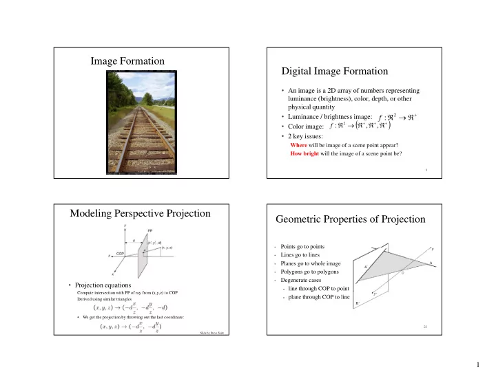
Image Formation Digital Image Formation

• An image is a 2D array of numbers representing
• An image is a 2D array of numbers representing

luminance (brightness), color, depth, or other physical quantity

• Luminance / brightness image:
• Color image:

2 k i



  2 : f

 

  

     , , :

2

f

• 2 key issues:

Where will be image of a scene point appear? How bright will the image of a scene point be?

2

Modeling Perspective Projection

• Projection equations

C i i i h PP f f ( ) COP Compute intersection with PP of ray from (x,y,z) to COP Derived using similar triangles

• We get the projection by throwing out the last coordinate:

Slide by Steve Seitz

Geometric Properties of Projection

• Points go to points

Points go to points

• Lines go to lines
• Planes go to whole image
• Polygons go to polygons
• Degenerate cases
• line through COP to point

21

g p

• plane through COP to line

2

Distant Objects are Smaller

22

Magnification = f/z

Tilted Objects are Foreshortened

24

Tilted Objects are Foreshortened

25

Parallel Lines Perpendicular to the Optical Axis

• Will be parallel in the

image

• Distant lines appear

closer together – “foreshortened”

26

Picture plane

3

In General, Parallel Lines Meet

Moving the image plane merely scales the image

27 28

Vanishing Points

picture plane eye vanishing point

Line parallel to scene line and passing through i l

• Vanishing point

y ground plane

• ptical center

29

Vanishing point

projection of a point “at infinity” Point in image beyond which projection of straight line cannot extend

Vanishing Points (2D)

picture plane eye vanishing point line on ground plane

30

4

Vanishing Points

image plane Eye vanishing point V

• Properties

An t o parallel lines ha e the same anishing point v

viewpoint C line on ground plane line on ground plane 31

Any two parallel lines have the same vanishing point v The ray from C through v is parallel to the lines An image may have more than one vanishing point

Vanishing lines

v1 v2

• M ltiple Vanishing Points

32

• Multiple Vanishing Points

Any set of parallel lines on a plane define a vanishing point The union of all of these vanishing points is the horizon line

• also called vanishing line

Note that different planes define different vanishing lines

Carlo Crivelli (1486) The Annunciation, with St. Emidius Perspective analysis of Crivelli’s Annunciation

5

Vanishing Lines

• Multiple Vanishing Points

35

p g

Any set of parallel lines on a plane define a vanishing point The union of all of these vanishing points is the horizon line

• also called vanishing line

Note that different planes define different vanishing lines

• For right-angled objects whose face normals are perpendicular to

the x, y, z coordinate axes, number of vanishing points = number

• f principal coordinate axes intersected by projection plane

Vanishing Points

y y y

y

x y x z y z x y x z y

z

One Point Perspective (z-axis vanishing point)

36

x z z x z

Two Point Perspective (z- and x-axis vanishing points) Three Point Perspective (z-, x-, and y-axis vanishing points)

Vanishing Points

l

each set of parallel lines

l

Good ways to spot faked

l

each set of parallel lines (= direction) meets at a different point

l

The vanishing point for this direction

l

Sets of parallel lines on the same plane lead to

l

Good ways to spot faked images

l

scale and perspective don’t work

l

vanishing points behave badly

l

supermarket tabloids are a t

37

p collinear vanishing points

l

The line is called the horizon for that plane great source

Masaccio’s “Trinity” (c. 1425-8)

• The oldest existing

example of linear ti i W t t perspective in Western art

• Use of “snapped” rope

lines in plaster

• Vanishing point below
• rthogonals implies

looking up at vaulted ceiling

6 Piero della Francesca, “Flagellation of Christ” (c. 1455)

• Carefully
• Carefully

planned

• Strong

sense of space

• Low eye
• Low eye

level

Leonardo da Vinci, “Last Supper” (c. 1497)

• Use of perspective to

direct viewer’s eye

• Strong perspective lines to

corners of image

Raphael, “School of Athens” (1510-11)

• Single-point

g p perspective

• Central
• Strong,

coherent space

Perspective Cues from Parallel Lines in the Scene

42

7

Perspective Cues

43

Perspective Cues

44

Comparing Heights

Vanishing Vanishing Point Point

45

Painters have used Heuristics to aid in Robust Perception of Perspective

“Make your view at least 20 times as far off as the

To minimize noticeable distortion, use shallow perspective:

Example: Leonardo’s Moderate Distance Rule

y f ff greatest width or height of the objects represented, and this will satisfy any spectator placed anywhere

• pposite to the picture.”
• - Leonardo

8 Example: Extreme Viewpoints Example: Extreme Viewpoints Perspective Perspective

Mantegna, Lamentation over the dead Christ, 1480

Ogden’s photo recreation of The dead Christ.

Example 2: Marginal View Example 2: Marginal View Distortion Distortion

Objects that are close to the viewer and at edge of field of view, are elongated by perspective projection Pinhole camera photo of a marginal sphere projection Plato (Leonardo) Aristotle Raphael, School of Athens, 1511 Heraclitus (Michaelangelo) Euclid (Bramante)

9

Z t Ptolomy Zoroaster Spheres should be elongated to be perspectively Detail of Raphael’s School of Athens be perspectively correct, but they are not

Leonardo’s Solution to the Problem Leonardo’s Solution to the Problem

“Make your view at least 20 times as far off as the greatest width or height of the objects width or height of the objects represented, and this will satisfy any spectator placed anywhere opposite to the picture.”

• - Leonardo

Pirenne’s pinhole camera photo of marginal columns

Camera Transformations using Homogeneous Coordinates

• Computer vision and computer graphics usually represent

points in Homogeneous coordinates instead of Cartesian coordinates

• Homogeneous coordinates are useful for representing

perspective projection, camera projection, points at infinity, etc.

• Cartesian coordinates (x, y) represented as Homogeneous

61

coordinates (wx, wy, w) for any scale factor w0

• Given 3D homogeneous coordinates (x, y, w), the 2D

Cartesian coords are (x/w, y/w). I.e., a point projects to w=1 plane

Homogeneous Coordinates

Converting to homogeneous coordinates:

homogeneous image coordinates homogeneous scene coordinates

Converting from homogeneous coordinates: g f g

Slide by Steve Seitz

10

The Projective Plane

• Geometric intuition

A point in the image is a ray in projective space from origin

(0,0,0)

(sx,sy,s) (x,y,1) y

• Each point (x,y) on the plane is represented by a ray (sx,sy,s)

– all points on the ray are equivalent: (x, y, 1)  (sx, sy, s)

image plane x z

Projective Lines

• What does a line in the image correspond to in

projective space?

• A line in the image is a plane of rays through origin

– all rays p = (x,y,z) satisfying: ax + by + cz = 0

 

 

           z y x c b a : notation vector in

• A line is also represented as a homogeneous 3-vector l

l p

2D Mappings

• 2D translation - 2 DOFs

   

• 2D rotation (counterclockwise about the origin) - 1 DOF

 

                     1 1 1 1 1 , , v u b a y x

T



    sin cos u  

       b v y a u x

• 2D rigid (Euclidean) transformation: translation and

rotation – 3 DOFs

            cos sin sin cos v u y v u x

                      1 1 cos sin sin cos ] 1 , , [ v u y x

T

   

2D Mappings (cont.)

• 2D scale - 2 DOFs
• Composite translation, rotation, scale (similarity

     v y u x  

                     1 1 ] 1 , , [ v u y x

T

  transformation) - 5 DOFs                         1 1 ) cos sin ( cos sin ) sin cos ( cos cos ] 1 , , [ v u b a b a y x

T

             

11

2D Mappings (cont.)

• Affine (linear) - 6 DOFs
• Projective (allows skewing) - 8 DOFs (a33 is a scale

factor)                      1 1 ] 1 , , [

23 22 21 13 12 11

v u a a a a a a y x

T

        

23 22 21 13 12 11

a v a u a y a v a u a x

   a v a u a                      1 ] 1 , , [

33 32 31 23 22 21 13 12 11

v u a a a a a a a a a y x

T

                 1 1

5 4 3 2 1 5 4 3 2 1

v a u a b v b u b y v a u a a v a u a x

Examples of 2D Transformations

Original Rigid Affine Projective

Properties of Transformations

• Projective
• Projective
• Preserves collinearity, concurrency, order of contact
• Affine (linear transformations)
• Preserves above plus parallelism, ratio of areas, …
• Similarity (rotation, translation, scale)

P b l ti f l th l

• Preserves above plus ratio of lengths, angle
• Euclidean (rotation and translation)
• Preserves above plus length, area

70

Using Homogeneous Coordinates

71

12

72 73

3D Mappings

• Cartesian coordinates (x, y, z)  (x, y, z, w) in

homogeneous coordinates g

• 4 x 4 matrix for affine transformations:

       

23 22 21 13 12 11 y x

t r r r t r r r t r r r

where rij specify aggregate rotation and scale change, and ti specify translation

      1

33 32 31 z

t r r r

• Projection is a matrix multiply using homogeneous

coordinates:

Perspective Projection

divide by third coordinate

This is known as perspective projection

• The matrix is the camera perspective projection matrix
• Can also formulate as a 4x4

divide by fourth coordinate

Slide by Steve Seitz

13

Perspective Projection

• How does multiplying the projection matrix by a

constant change the transformation?

Homographies

• Perspective projection of a plane

Lots of names for general plane-to-plane transformations:

• homography texture map colineation planar projective map
• homography, texture-map, colineation, planar projective map

Modeled as a 2D warp using homogeneous coordinates

sx' * * * x sy' * * * y s * * * 1                               

H  H p p To apply a homography H

• Compute p = Hp

(regular matrix multiply)

• Convert p from homogeneous to image coordinates

– divide by s (third) coordinate

Camera Parameters

A camera is described by several parameters

• Translation T of the optical center from the origin of world coords
• Rotation R of the image plane
• focal length f, principle point (x’c, y’c) , pixel size (sx, sy)

Projection equation

• The projection matrix models the cumulative effect of all parameters

U f l t d i t i f ti

ΠX x

                                   1 * * * * * * * * * * * * Z Y X s sy sx

g , p p p (

c, y c) , p

(

x, y)

• blue parameters are called “extrinsics,” red are “intrinsics”
• Useful to decompose into a series of operations

                                       1 1 1 1 1 1 ' '

3 1 1 3 3 3 3 1 1 3 3 3 x x x x x x c y c x

y fs x fs

T I R Π

projection intrinsics rotation translation

identity matrix

Note: Can also add other parameters to model lens distortion K