7. Functions of more than one variable Most functions in nature - PDF document

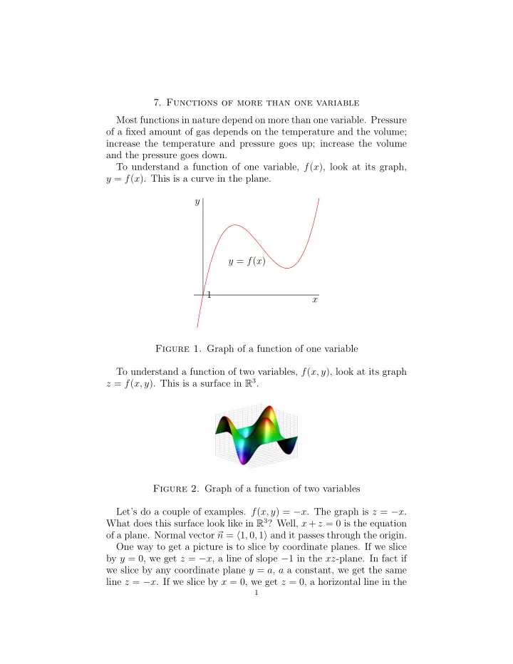
7. Functions of more than one variable Most functions in nature depend on more than one variable. Pressure of a fixed amount of gas depends on the temperature and the volume; increase the temperature and pressure goes up; increase the volume and the pressure goes down. To understand a function of one variable, f ( x ), look at its graph, y = f ( x ). This is a curve in the plane. y y = f ( x ) 1 x Figure 1. Graph of a function of one variable To understand a function of two variables, f ( x, y ), look at its graph z = f ( x, y ). This is a surface in R 3 . Figure 2. Graph of a function of two variables Let’s do a couple of examples. f ( x, y ) = − x . The graph is z = − x . What does this surface look like in R 3 ? Well, x + z = 0 is the equation of a plane. Normal vector � n = � 1 , 0 , 1 � and it passes through the origin. One way to get a picture is to slice by coordinate planes. If we slice by y = 0, we get z = − x , a line of slope − 1 in the xz -plane. In fact if we slice by any coordinate plane y = a , a a constant, we get the same line z = − x . If we slice by x = 0, we get z = 0, a horizontal line in the 1

yz -plane. If we slice by x = 1, we get z = − 1, a different horizontal line. How about f ( x, y ) = 1 − x 2 − y 2 ? If we slice by y = 0, we get z = 1 − x 2 , an upside down parabola. If we slice by y = 1, we get z = − x 2 , another upside down parabola. Similarly if we slice by y = a , we get the parabola, z = − x 2 − a 2 . By symmetry in x and y , we get the same picture if we slice by x = a . How about if we fix z ? Then x 2 + y 2 = 1 − z . So we only get a non- empty slice, if we take z ≤ 1. If z = 0, we get the circle x 2 + y 2 = 1. If we increase z , we get circles of smaller radii. If we decrease z they get bigger. In fact the graph is a paraboloid. Figure 3. Paraboloid One way to get a picture of the graph is to look at the contour lines. These are lines in the xy -plane of constant height. Formally, they are the solutions to the equation f ( x, y ) = c, where c is fixed. The contour lines of f ( x, y ) = 1 − x 2 − y 2 are concentric circles centred at the origin: What does x 2 + y 2 , � z = look like? Well the contour lines are circles, so it looks like a paraboloid. But if we cut by coordinate planes, we get a different picture. If we √ take the plane y = 0, we get z = x 2 , or what comes to the same thing x 2 + y 2 is the � z = | x | . The graph of this look like a V. In fact z = graph of a cone. It is not hard to see that z = x 2 + y 2 is another paraboloid. It is the same story as z = 1 − x 2 − y 2 . The contour lines are the circles x 2 + y 2 = c . Cutting by coordinate hyperplanes, we get parabolas, but this time the right way up, so that the graph of z = x 2 + y 2 is a paraboloid the other way up to z = 1 − x 2 − y 2 . 2

0.3 0.1 0.4 0.2 Figure 4. Contour lines of paraboloid What does z = y 2 − x 2 , look like? Well the contour lines are hyperbolae: -0.1 0.3 0.2 0.4 -0.2 -0.3 -0.5 0.1 -0.4 -0.4 0.1 -0.5 -0.3 -0.2 0.4 0.2 0.3 -0.1 Figure 5. Contour lines for y 2 − x 2 How about if we take cross sections? Fix x = a , we get parabolas z = y 2 − a 2 . Fix y = a , we get upside down parabolas z = a 2 − x 2 . The graph of this function is called a saddle point: One way to understand a function of one variable is to differentiate. The derivative is the slope of the tangent line. 3

Figure 6. Saddle point If we have a function of two variables, there are two obvious deriva- tives. We could fix y and vary x , to get a partial derivative � f x ( x 0 , y 0 ) = ∂f f ( x 0 + ∆ x, y 0 ) − f ( x 0 , y 0 ) � = lim . � ∂x ∆ x ∆ x → 0 � x = x 0 ,y = y 0 Similarly, we can fix x and vary y . � f y ( x 0 , y 0 ) = ∂f f ( x 0 , y 0 + ∆ y ) − f ( x 0 , y 0 ) � = lim . � ∂y ∆ y ∆ y → 0 � x = x 0 ,y = y 0 f x is the slope of the tangent line if you cut by the plane y = y 0 ; f y is the slope of the tangent line to if you cut by the plane x = x 0 . It is straightforward to calculate partial derivatives. Let f ( x, y ) = x 2 y − sin( x + y 2 ). f y = x 2 − 2 y cos( x + y 2 ) . f x = 2 xy − cos( x + y 2 ) and ∂ (ln( x cos y )) x cos y = 1 1 = cos y x, ∂x and ∂ (ln( x cos y )) 1 = − x sin y x cos y = − tan y. ∂y We can use partial derivatives to estimate the change in f , if we change x and y by a small amount. ∆ f ≈ f x ∆ x + f y ∆ y. In fact, we can calculate the tangent plane at a point ( x 0 , y 0 , z 0 ), where z 0 = f ( x 0 , y 0 ). One way to calculate the tangent plane is to use the approximation formula, ( † ) z − z 0 = f x ( x 0 , y 0 )( x − x 0 ) + f y ( x 0 , y 0 )( y − y 0 ) . In fact the approximation formula works by approximating ∆ f by using linear approximation. The tangent plane is the best linear approxima- tion to the function f . 4

The tangent plane is the plane which should contain the tangent line to any curve in the graph. You can get two curves easily, either by fixing y and varying x or by fixing x and varying y . These are the curves you get by cutting by either the plane y = y 0 or the plane x = x 0 . The tangent line to the first curve is z − z 0 = f x ( x 0 , y 0 )( x − x 0 ) , and the tangent line to the second curve is z − z 0 = f y ( x 0 , y 0 )( y − y 0 ) . Visibly ( † ) contains both tangent lines. 5