Digital imaging and image processing Review Final Exam Monday - PowerPoint PPT Presentation
Digital imaging and image processing Review Final Exam Monday June 11th at 8am Digital Data Pixels Digital Sensors (a) Single sensing element. (b) Line sensor. (c) Array sensor. Digital Image Grayscale image Bit depth
Digital imaging and image processing Review Final Exam Monday June 11th at 8am
Digital Data
Pixels
Digital Sensors (a) Single sensing element. (b) Line sensor. (c) Array sensor.
Digital Image
Grayscale image
Bit depth • Binary: 0 and 1 • 8 bit: 0 up to (2^8 =) 256 • 16 bit: 0 up to (16^2 =) 65,536 • 32 bit: 0 up to (32^2 =) 4,294,967,296 • Color: RGB contains a red, green and blue matrix of the bit depth specified
Image displayed in 32, 16, 8, 4, and 2 intensity levels.
Saturation
Forming a vector
Color Images blue green red
Color sensor: Bayer pattern
We lose light
Dichroic Mirrors, Multiple Cameras • N
Image Display Simplest contrast adjustment: Set Min, Max of display
More powerful methods to improve contrast Retinex—Examples—X-rays
• Make image “better” for a specific application In image space – The idea of “better” is somewhat subjective • Make image “better” for a specific application • – The idea of “better” is somewhat subjective – – • We distinguish two domains: – Spatial or Pixel domain: ( , ) or ( , ) f x y f m n • – Frequency Domain: ( , ) or ( , ) F w w F u v – x y – • – – Pixel 4-Neighbors 8-Neighbors
Operations • Element-wise (pixel by pixel) vs. Matrix operations • Single-pixel vs neighborhood: • Single-pixel: grab e.g. the value of the one nearest pixel) • Neighborhood (calculate and use e.g. the average / max / median / min or other calculated value of the nearest neighbors)
Simplest form of processing: Point Processing Pixel T r � ( , ) s � f m n ( r ) T 255 No change S=T(r) Image “negative”: s=L -1-r Thresholding 0 255 r Black � � � � • � � • � � � � Narrow range of “dark” gets mapped to broad range of “gray”
Inverse lookup table (a) 8-bit image. (b) Intensity transformation function used to obtain the digital equivalent of a “photographic” negative of an 8-bit image. The arrows show transformation of an arbitrary input intensity value z into its corresponding output value s0. (c) Negative of (a) obtained using (b)
Better visibility for display / diagnosis
Binary • Small storage • Easier to apply some operations
� � Image “negative”: s=L Simplest form of processing: Point Processing Pixel T r � ( , ) s � f m n ( r ) T Common Examples: 255 � � 0 . 1 • Dynamic Range Compression � � ( ) log( 1 ) T r c r s • Gamma Correction � � ( ) T r cr � � 10 Narrow range of “dark” gets mapped to broad range of “gray” 0 255 r Black
Gamma Correction • Nonlinear response of CRT’s and imagers • commands to the CRT are “predistorted” Luminance � � L U � � � 1 . 8 2 . 5 0 Applied/Measured Voltage (U)
• Nonlinear response of CRT’s and imagers • commands to the CRT are “predistorted” � � � � �
Scaling
Log scale display
Synthetic lookup tables Inverse “Red Hot” in FIJI Chasing the right one can make it easier to see stuff — and to get published…
Histogram Processing: • Distribution of gray-levels can be judged by measuring a Histogram 15 9 7 5 Histogram: Graylevel • • • • •
Histograms
Histogram manipulation Illustration of the mean and standard deviation as functions of image contrast. (a)-(c) Images with low, medium, and high contrast, respectively. (Original image courtesy of the National Cancer Institute.)
Example:
Histogram Equalization • Make it flat and spread it out • This is a nonlinear operation
• • • – – Histogram Equalization: Cont.’d – • • � � � – – • – – •
Color Histogram
Spatial filtering • In image space • In frequency space
Image size / Sampling
Aliasing
Nyquist sampling = twice the frequency
Aliasing • (Image downsized around four times)
Re-sampling: Change size by interpolation (a) Image reduced to 72 dpi and zoomed back to its original 930 dpi using nearest neighbor interpolation. (b) Image reduced to 72 dpi and zoomed using bilinear interpolation. (c) Same as (b) but using bicubic interpolation.
Average when downsizing? • Edges lose contrast if you average but result is smoother
Convolution Defining convolution • Let f be the image and g be the kernel. The output of convolving f with g is denoted f * g . � � � � � ( )[ , ] [ , ] [ , ] f g m n f m k n l g k l , k l f • Convention: kernel is “flipped” • MATLAB: conv2 vs. filter2 (also imfilter) Source: F. Durand • • •
• � � � � � • Convention: kernel is “flipped” • Convolution Key properties • Linearity: filter( f 1 + f 2 ) = filter( f 1 ) + filter( f 2 ) • Shift invariance: same behavior regardless of pixel location: filter(shift( f )) = shift(filter( f )) • Theoretical result: any linear shift-invariant operator can be represented as a convolution
• • – = ‘full’: output size is sum of sizes of f and g – = ‘same’: output size is same as f – = ‘valid’: output size is difference of sizes of f Convolve • “Drag-and-Stamp” – To compute all pixel values in the output image, we need to fill in a “border” Mask dimension = 2M+1 Border dimension = M
Spatial Filtering: Blurring • Example Averaging Mask: 1 1 1 1/9 1 1 1 1 1 1 • � � � � � � � � � � � �
Image Enhancement:Spatial Filtering Operation • Idea: Use a “mask” to alter pixel values according to local operation • Aim: (De)-Emphasize some spatial frequencies in the image.
Image Enhancement:Spatial Filtering Operation • An important point: Edge Effects (Ex.: 5x5 Mask) – How to fill in a “border” d c a b c d • Zeros (Ringing) • Replication (Better) b a a b • Reflection (“Best”) a b b a c d c d • Procedure: – Replicate row-wise – Replicate column-wise – Apply filtering – Remove borders • – – – • • imfilter(f, g, ‘circular’) • imfilter(f, g, ‘replicate’) • imfilter(f, g, ‘symmetric’)
• – – – • • • • Image Enhancement:Spatial Filtering Operation 5x5 Blurring with 0-padding 5x5 Blurring with reflected padding
Gaussian Kernel 0.003 0.013 0.022 0.013 0.003 0.013 0.059 0.097 0.059 0.013 0.022 0.097 0.159 0.097 0.022 0.013 0.059 0.097 0.059 0.013 0.003 0.013 0.022 0.013 0.003 5 x 5, � = 1 fspecial(‘gauss’,5,1) • Constant factor at front makes volume sum to 1 (can be ignored, as we should re-normalize weights to sum to 1 in any case) •
� fspecial(‘gauss’,5,1) • Choosing kernel width • Gaussian filters have infinite support, but discrete filters use finite kernels
• σ Example: Smoothing with a Gaussian
Mean vs. Gaussian filtering • Remove “high frequency” components • – – σ σ √2 • –
Gaussian filters • Remove “high - frequency” components from the image (low-pass filter) • Convolution with self is another Gaussian – So can smooth with small-width kernel, repeat, and get same result as larger-width kernel would have – Convolving two times with Gaussian kernel of width σ is same as convolving once with kernel of width σ √2 • Separable kernel – Factors into product of two 1D Gaussians
Use this to sharpen! • What does blurring take away? – = detail smoothed (5x5) original Let’s add it back: + α = original detail sharpened
More on Linear Operations: Sharpening Filters • Sharpening filters use masks that typically have + and – numbers in them. • They are useful for highlighting or enhancing details and high-frequency information (e.g. edges) • They can (and often are) based on derivative- type operations in the image (whereas smoothing operations were based on “integral” type operations) • • � � � � � � � � � � � � � � �� �� � � � � � �� �� �� �� � � � � � • • � �
• – • • smoothing operations were based on “integral” Derivatives Differentiation and convolution • We could approximate • Recall, for 2D function, this as f(x,y): � � � f x n , y � � � � � � � f � f f x � � , y �� �� � x � f x n � 1 , y � f x , y � x � lim �� �� �� �� � � � x � � 0 • which is obviously a • This is linear and shift convolution with kernel invariant, so must be the result of a convolution. -1 1 � �
Recommend
More recommend
Explore More Topics
Stay informed with curated content and fresh updates.
