The Digital Image What is a Digital Image? How to Make an Image a - - PDF document

Computational Photography

CS 4475/6475 Maria Hybinette

1 Maria Hybinette

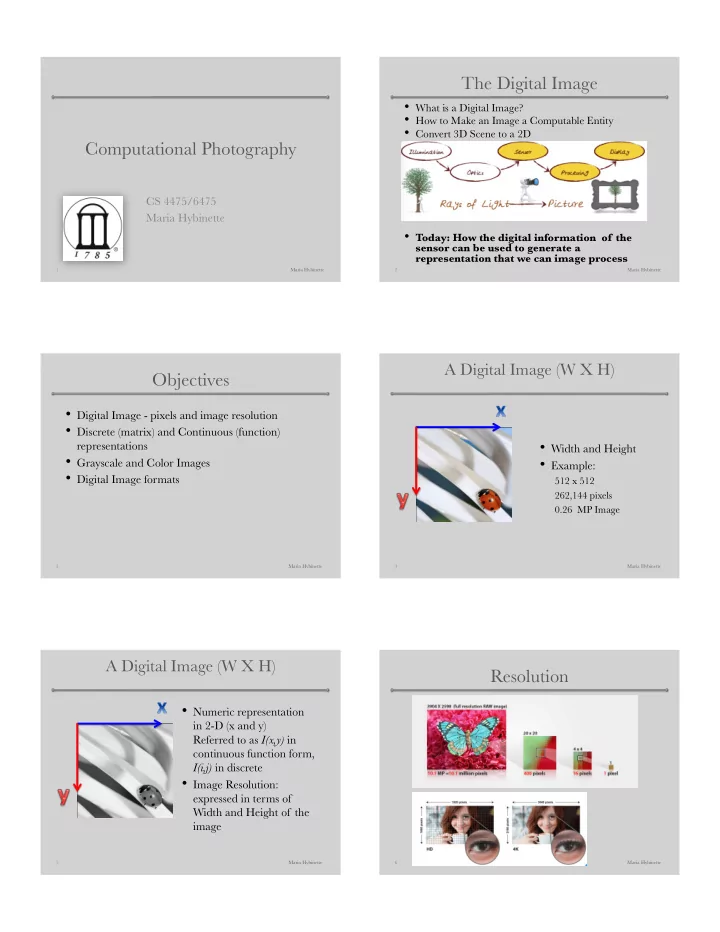
The Digital Image

• What is a Digital Image?
• How to Make an Image a Computable Entity
• Convert 3D Scene to a 2D
• ]
• Today: How the digital information of the

sensor can be used to generate a representation that we can image process

2 Maria Hybinette

Objectives

• Digital Image - pixels and image resolution
• Discrete (matrix) and Continuous (function)

representations

• Grayscale and Color Images
• Digital Image formats

Maria Hybinette 3

A Digital Image (W X H)

• Width and Height
• Example:

512 x 512 262,144 pixels 0.26 MP Image

Maria Hybinette 4

A Digital Image (W X H)

• Numeric representation

in 2-D (x and y) Referred to as I(x,y) in continuous function form, I(i,j) in discrete

• Image Resolution:

expressed in terms of Width and Height of the image

Maria Hybinette 5

Resolution

Maria Hybinette 6

Pixel

• A “picture element”that contains the light intensity

at some location

• (i,j) in the image

Maria Hybinette 7

Characteristics of a Digital Image

• A two-dimensional array of pixels and respective

intensities

• Image can be represented as a Matrix

Intensity Values range from 0 = Black to 255 = White

Maria Hybinette 8

Common data types

• Data types used to store pixel values:

– unsigned char – Uint8 – unsigned char 8bit – 2^n (2^1, 2^2, … 2^8) [2^8 = 256]

Maria Hybinette 9

Digital Image is a Function

Maria Hybinette 10

x y

Con'nuous Signal Discrete Signal

Digital Image is a Function

• Typically, the functional operation requires discrete values

Sample the two-dimensional (2D) space on a regular grid Quantize each sample (rounded to “nearest integer”)

• Matrix of integer values (Range: 0-255)

Maria Hybinette 11

Black/White Digital Image: An Example

• Revisit

Maria Hybinette 12

Image Statistics

• Digital Image Statistics
• Pixel Counts
• Image Histogram
• Image statistics - average, median, mode

Scope - entire image or smaller windows/regions

• Histogram - distribution of pixel intensities in the image
• Can be separate for each channel, or region-based too

Maria Hybinette 13

Histogram

• Underexposed originally left (made it grey)
• Corrected on the right

14 15

• Overexposed: clipped/blown channels

Contrast

• Narrow range low contrast e.g., (fog no texture on the

left)

• Broad range, high contras e.g., (texture water with a

range of tones).

16

Impossibilities

17

8 Stops

Bad Histograms?

18

How much latitude in Camera?

• Nine stops (each stops is double in brightness from its

neighbor) contrast range, plus all black and all white

– (12 stops Hasselblad, 10 stops Nikon D3X)

• Seven stop contrast range, plus all black and all white
• Five stop contrast range, plus all black and all white

19

h)p://www.forphotography.com/how-tos/zone/zone1.html

Color Digital Image: An Example

• Color image = 3 color channels (images, with their own

intensities) blended together

• Makes 3D data structure of size: Width X Height X

Channels Each pixel has therefore 3 intensities: Red (R), Green (G), Blue (B)

Maria Hybinette 20

Red Channel Green Channel Blue Channel

Digital Image Formats

• Raster image formats store a series of colored dots

“pixels”

• Number of bits for each pixel represents the depth
• f color

– 1 bit-per-pixel: 2 colors (black or white, binary) – 4 bits-per-pixel: 16 colors – 8 bits-per-pixel: 256 different colors {2^8}

• One per channel {24 bits} {8+8+8}

– Usually means 8 bits per color

Maria Hybinette 21

Digital Image Formats

• Images can also be 16, 24, 32 bits-per-pixel:
• 24 bits per pixel usually means 8 bits per color
• At the two highest levels, the pixels themselves can

carry up to 16,777,216 different colors

• Common raster image formats:
• GIF, JPG, PPM, TIF, BMP

, etc.

• Will discuss Camera RAW format later

Maria Hybinette 22

Exercise

• Read and Write Image
• import cv2
• img = cv2.imread('input.png')
• cv2.imwrite('output.png', img)
• print cv2img
• cv2greyimg = cv2.cvtColor( cv2img,

cv2.COLOR_RGB2GRAY )

• print cv2greyimg
• width = data_array.shape[1]

Maria Hybinette 23

• Break then we will go over

– Point processes (we will use slides from last year0

Maria Hybinette 24

Wednesday

• Blend Modes
• Image Smoothing
• Start on Image Filters

Maria Hybinette 25

Part 2: Image Processing and Filtering

• Pont-process Computations on an Image
• How to combine intensities from 2 images?

Maria Hybinette 26

Lesson Objectives

• Point-process Computations:
• Add/Subtract Images
• α-blending & its applications
• Image Histograms

Maria Hybinette 27

Review: Digital Image

• How to obtain discrete values?

Sample the two-dimensional (2D) space on a regular grid Quantize each sample (round to “nearest integer”)

• Result: Matrix of integer values (range, e.g.:

0-255)

Maria Hybinette 28

Arithmetic Practice

• On the data structure

Maria Hybinette 29

Pixel/Point Arithmetic: An Example

• Subtraction
• Binary Result

Maria Hybinette 30

Pixel Operations: Another Example

• 3 Images Added Together
• Step 1. Too bright
• Step 2. Weigh (normalize) their contribution to the

final image

Maria Hybinette 31

Alpha Blending

• .34 x CD+.34 x AE+.34 x LD=
• Transparency (Conversely, Opacity!)

Usually represented as: α α varies from 0 to 1.0 (0=invisible, 1.0=fully visible)

• RGB αRGB

Maria Hybinette 32

Part 3:

• Blend two pixels from two images
• Examples

– averages

• fblend(a,b) = (a+b) /2
• fblend(a,b) = b

– Top layer in photoshop or gimp

Maria Hybinette 33

Blending Modes (simple)

• Divide (‘standardize) pixel value first to be

between [0, 1] à 0 (black, 0) – 1(white, 255)

– Brightens photos if standardized, otherwise it would darken.

• Addition (too many whites)
• Subtract (too many blacks)
• Difference (subtract with scaling)
• Darken: fblend(a, b) = min(a, b) for RGB
• Lighten: fblend(a, b) = max(a, b) for RGB

Maria Hybinette 34

Advanced Modes

• Photoshop uses standardized numbers

White (255) becomes 1, black (0) is 0

» .80 (light gray) » .50 (middle gray) » .40 (dark gray)

• Multiply fblend(a,b) = ab

– .8*.8 = .64 darker than original – .4*.4 = .16 darker

• Screen fblend(a,b) = 1 - (1 – a)(1-b)

– brighter f(.8,.8) = 1 - (.2)(.2) = 1-.04= . 96

Maria Hybinette 35

Advanced Modes

• Overlay fblend(a, b) = 2 ab if a < 0.5 (dark)

1 - 2(1 – a)(1-b)

– Top looks like “multiply” (when a < .5, darker than middle gray), and – “screen” when a is greater (or brighter than middle gray). – Pulls the values further away from middle gray. – Recall 0 is black .5 grey and 1 is white when standardized.

Maria Hybinette 36

Commuted Blend Model

• Apply the ‘other blend mode’ in reveres order you

get the same result.

• Overlay and Hard Light

– Overlay(a, b) = HardLight (b, a)

• Luminosity and Color

– Luminosity(a, b) = HardLight (b, a)

Maria Hybinette 37

Other Modes for Reference

Darkens:

• Burn Tool darkens an area without affecting saturation or

color (different from the below modes).

• Color Burn

fblend(a,b) = 1-(1-b)/a

(SP8)

• Linear Burn

fblend(a,b) = a+b-1

(SP8)

Lightens:

• Dodge Tool: Ligthens specified area different from below

modes.

• Color Dodge

fblend(a,b) = b/(1-a) (SP8)

• Linear Dodge

fblend(a,b) = a+b (SP8)

Maria Hybinette 38

h)p://photoblogstop.com/photoshop/photoshop-blend-modes-explained

Sources & Inspiration

Contributors of Course Material:

• Irfan Essa & Frank Dellaert (Georgia Tech)

– Also early adopters

• Marc Levoy (Stanford)– taught computational

photography since 2002: – A leader in the field : Frankecamera

• Frédo Durand (MIT)
• Jack Tumblin (Northwestern)
• Wikipedia
• http://www.all-art.org/

history658_photography1.html

• “Photography”, London, Stone, Upton

Maria Hybinette 39