SLIDE 1
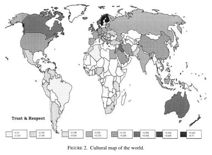
Figure 2. Cultural map of the world.
SLIDE 2 TABLE I TRUST, CIVIC COOPERATION, AND ECONOMIC PERFORMANCE, 1980–1992 Equation 1 2 3 4 5 6 7 Method OLS OLS OLS OLS 2SLS OLS OLS Dependent Investment/GDP variable Growth 1980–1992 1980–1992 Constant 0.935 10.476 9.593 2.829 1.037 9.617 23.893 (1.280) (4.730) (4.520) (1.895) (1.898) (3.820) (11.998) GDP80 0.361 0.273 0.375 0.152 0.366 0.162 0.273 (0.131) (0.126) (0.127) (0.274) (0.127) (0.403) (0.364) PRIM60 6.192 5.930 7.061 4.818 6.270 11.655 13.030 (1.051) (1.164) (1.224) (1.709) (1.759) (3.558) (3.274) SEC60 2.194 3.457 1.648 1.256 2.085 0.431 0.495 (1.632) (1.543) (1.485) (1.930) (2.133) (8.286) (7.067) PI80 3.693 3.117 3.535 3.930 3.713 4.435 3.170 (0.867) (1.100) (0.935) (0.755) (0.809) (1.993) (2.154) TRUST 0.082 0.076 0.192 0.086 0.146 (0.030) (0.030) (0.060) (0.039) (0.078) CIVIC 0.272 0.207 0.872 (0.098) (0.092) (0.301) TRUST*GDP80 0.013 (0.006)
.55 .44 .56 .60 .52 .37 .38 SEE 1.37 1.52 1.35 1.29 1.37 4.43 4.38 Mean, D.V. 1.45 1.45 1.45 1.45 1.45 22.4 22.4
White [1980]-corrected standard errors are in parentheses. Instruments for TRUST in equation 5 include law students/total postsecondary students, Sullivan’s homogeneity indicator, GDP80, SEC60, PRIM60, and PI80. Note that R2 and SEE do not have their usual interpretations in 2SLS. R2’s without social capital variables are .41 (growth) and .33 (inv./GDP). All equations have 29 observations.
Knack and Keefer (QJE 1997)
SLIDE 3 Table 4. Trust and ancestors’ countries—probit estimates.
Trust Dependent variable (1) (2) (3) (4) (5) (6) (7) Trust from 2000 WWS 0.55 0.67 (0.22)** (0.21)***
0.06 0.06 0.07 0.05 0.06 (0.02)*** (0.02)*** (0.02)** (0.02)*** (0.01)*** Polity2 up to 1900 0.05 (0.02)*** Per capita income 1870 0.00 (0.08) Per capita income 1930 –0.03 –0.16 –0.24 (0.08) (0.10) (0.08)*** Primary school enr. 1910 0.52 0.50 (0.18)*** (0.16)*** Observations 4267 4267 4267 3907 3907 3520 3520 Pseudo R2 0.08 0.09 0.08 0.09 0.09 0.09 0.10 Notes: Robust standard errors in parentheses, clustered by country of origin of ancestors. All regressions include the following controls: Gender; family income in constant dollar (base = 1986); dummy variables if completed high school, if completed college, if working, if unemployed, for age over 65, for age under 25, if married, for having at least one child, if Catholic, if Protestant, if Jewish, if father attended primary school, if mother attended primary school, if father attended college, if mother attended college, for living in urban area; number of grandparents born outside US; dummy variables for survey’s decade (1980s, 1990s or after year 2000); dummy variables for metropolitan area or county of residence (258 dummies altogether).
∗Significant at 10%; ∗∗significant at 5%; ∗∗∗significant at 1%.
SLIDE 4 Table 5. Culture and Governance, cross-country OLS estimates. GADP & Bureaucratic quality Dependent variable (1) (2) (3) (4) Trust 0.468 (0.218)** Respect 0.522 (0.263)* Trust & Respect 0.359 0.279 (0.144)** (0.073)*** Primary education in 1930 0.007 0.007 0.006 0.000 (0.001)*** (0.001)*** (0.001)*** (0.001) Income in 1980–2000 0.214 (0.033)*** Observations 57 57 57 56 Adjusted R2 0.66 0.64 0.68 0.86
Notes: Robust standard errors in parentheses. Other included covariates: Dummy variables for French and UK legal origin.
∗Significant at 10%; ∗∗significant at 5%; ∗∗∗significant at 1%.
SLIDE 5 Table 6. Language and values inside countries, from individual respondents. Trust Respect Trust & Respect Dependent variable (1) (2) (3) 2nd person Differentiation –0.22 –0.25 –0.24 (0.09)** (0.04)*** (0.04)*** (–0.06) (–0.08) No pronoun drop 0.18 0.05 0.12 (0.10)* (0.07) (0.06)** (0.05) (0.02) Estimation Probit Probit Ordered Probit Observations 8640 8640 8640 Pseudo R2 0.07 0.03 0.04
Notes: Robust standard errors in the first parentheses, clustered by country. Marginal effects in the second parenthesis (estimated at the sample average for all variables). Other covariates: dummy variables for gender, age (over 65 and under 25 years of age), being married, having no
- children. Country fixed effects and dummy variables for each wave are always included.
∗Significant at 10%; ∗∗significant at 5%; ∗∗∗significant at 1%.
SLIDE 6 Table 8. Values and Governance—2SLS estimates. GADP & Bureaucratic quality Dependent variable (1) (2) (3) (4) Trust & Respect 0.57 0.52 0.60 1.39 (0.22)** (0.21)** (0.17)*** (0.39)*** Also control for Income in 1980–2000 Constraints on Executive 1960–2000 Settler’s Mortality Observations 48 47 48 21
Notes: Robust standard errors in parentheses. Instruments for Trust & Respect: Language. Other covariates included in columns 1–3: Primary education in 1930, UK and French legal origin. Column 4 includes no other covariates.
∗Significant at 10%; ∗∗significant at 5%; ∗∗∗significant at 1%.
SLIDE 7
Panel A. Transatlantic slave trade
Atlantic slave exports 1 – 100,000 100,001 – 500,000 500,001 – 1,000,000 1,000,001 – 4,000,000
SLIDE 8
Indian slave exports
Panel B. Indian Ocean slave trade
1 – 1,000 1,001 – 50,000 50,001 – 100,000 100,001 – 1,000,000
SLIDE 9
SLIDE 10 TABLE III RELATIONSHIP BETWEEN SLAVE EXPORTS AND INCOME Dependent variable is log real per capita GDP in 2000, ln y (1) (2) (3) (4) (5) (6) ln(exports/area) −0.112∗∗∗ −0.076∗∗∗ −0.108∗∗∗ −0.085∗∗ −0.103∗∗∗ −0.128∗∗∗ (0.024) (0.029) (0.037) (0.035) (0.034) (0.034) Distance from 0.016 −0.005 0.019 0.023 0.006 equator (0.017) (0.020) (0.018) (0.017) (0.017) Longitude 0.001 −0.007 −0.004 −0.004 −0.009 (0.005) (0.006) (0.006) (0.005) (0.006) Lowest monthly −0.001 0.008 0.0001 −0.001 −0.002 rainfall (0.007) (0.008) (0.007) (0.006) (0.008) Avg max humidity 0.009 0.008 0.009 0.015 0.013 (0.012) (0.012) (0.012) (0.011) (0.010) Avg min −0.019 −0.039 −0.005 −0.015 −0.037 temperature (0.028) (0.028) (0.027) (0.026) (0.025) ln(coastline/area) 0.085∗∗ 0.092∗∗ 0.095∗∗ 0.082∗∗ 0.083∗∗ (0.039) (0.042) (0.042) (0.040) (0.037) Island indicator −0.398 −0.150 (0.529) (0.516) Percent Islamic −0.008∗∗∗ −0.006∗ −0.003 (0.003) (0.003) (0.003) French legal origin 0.755 0.643 −0.141 (0.503) (0.470) (0.734) North Africa 0.382 −0.304 indicator (0.484) (0.517) ln(gold prod/pop) 0.011 0.014 (0.017) (0.015) ln(oil prod/pop) 0.078∗∗∗ 0.088∗∗∗ (0.027) (0.025) ln(diamond −0.039 −0.048 prod/pop) (0.043) (0.041) Colonizer fixed Yes Yes Yes Yes Yes Yes effects Number obs. 52 52 42 52 52 42 R2 .51 .60 .63 .71 .77 .80
- Notes. OLS estimates of (1) are reported. The dependent variable is the natural log of real per capita
GDP in 2000, ln y. The slave export variable ln(exports/area) is the natural log of the total number of slaves exported from each country between 1400 and 1900 in the four slave trades normalized by land area. The colonizer fixed effects are indicator variables for the identity of the colonizer at the time of independence. Coefficients are reported with standard errors in brackets. ∗∗∗, ∗∗, and ∗ indicate significance at the 1%, 5%, and 10% levels.
SLIDE 11
SLIDE 12 TABLE IV ESTIMATES OF THE RELATIONSHIP BETWEEN SLAVE EXPORTS AND INCOME (1) (2) (3) (4) Second Stage. Dependent variable is log income in 2000, ln y ln(exports/area) −0.208∗∗∗ −0.201∗∗∗ −0.286∗ −0.248∗∗∗ (0.053) (0.047) (0.153) (0.071) [−0.51, −0.14] [−0.42, −0.13] [−∞, +∞] [−0.62, −0.12] Colonizer fixed No Yes Yes Yes effects Geography controls No No Yes Yes Restricted sample No No No Yes F-stat 15.4 4.32 1.73 2.17 Number of obs. 52 52 52 42 First Stage. Dependent variable is slave exports, ln(exports/area) Atlantic distance −1.31∗∗∗ −1.74∗∗∗ −1.32∗ −1.69∗∗ (0.357) (0.425) (0.761) (0.680) Indian distance −1.10∗∗∗ −1.43∗∗∗ −1.08 −1.57∗ (0.380) (0.531) (0.697) (0.801) Saharan distance −2.43∗∗∗ −3.00∗∗∗ −1.14 −4.08∗∗ (0.823) (1.05) (1.59) (1.55) Red Sea distance −0.002 −0.152 −1.22 2.13 (0.710) (0.813) (1.82) (2.40) F-stat 4.55 2.38 1.82 4.01 Colonizer fixed No Yes Yes Yes effects Geography controls No No Yes Yes Restricted sample No No No Yes Hausman test .02 .01 .02 .04 (p-value) Sargan test (p-value) .18 .30 .65 .51
- Notes. IV estimates of (1) are reported. Slave exports ln(exports/area) is the natural log of the total number
- f slaves exported from each country between 1400 and 1900 in the four slave trades normalized by land area.
The colonizer fixed effects are indicator variables for the identity of the colonizer at the time of independence. Coefficients are reported, with standard errors in brackets. For the endogenous variable ln(exports/area), I also report 95% confidence regions based on Moreira’s (2003) conditional likelihood ratio (CLR) approach. These are reported in square brackets. The p-value of the Hausman test is for the Wu–Hausman chi-squared
- test. ∗∗∗, ∗∗, and ∗ indicate significance at the 1%, 5%, and 10% levels. The “restricted sample” excludes island
and North African countries. The “geography controls” are distance from equator, longitude, lowest monthly rainfall, avg max humidity, avg min temperature, and ln(coastline/area).
SLIDE 13 Table 1—OLS Estimates of the Determinants of Trust in Neighbors Dependent variable: Trust of neighbors Slave exports (thousands) Exports/ area Exports/ historical pop ln (1 + exports) ln (1 + exports/ area) ln (1 + exports/ historical pop) (1) (2) (3) (4) (5) (6) Estimated coeffjcient −0.00068 −0.019 −0.531 −0.037 −0.159 −0.743 [0.00014] [0.005] [0.147] [0.014] [0.034] [0.187] (0.00015) (0.005) (0.147) (0.014) (0.034) (0.187) {0.00013} {0.005} {0.165} {0.015} {0.034} {0.212} Individual controls Yes Yes Yes Yes Yes Yes District controls Yes Yes Yes Yes Yes Yes Country fjxed effects Yes Yes Yes Yes Yes Yes Number of observations 20,027 20,027 17,644 20,027 20,027 17,644 Number of ethnicities 185 185 157 185 185 157 Number of districts 1,257 1,257 1,214 1,257 1,257 1,214 R2 0.16 0.16 0.15 0.15 0.16 0.15 Notes: The table reports OLS estimates. The unit of observation is an individual. Below each coeffjcient three standard errors are reported. The fjrst, reported in square brackets, is standard errors adjusted for clustering within ethnic groups. The second, reported in parentheses, is standard errors adjusted for two- way clustering within ethnic groups and within districts. The third, reported in curly brackets, is T. G. Conley (1999) standard errors adjusted for two-dimensional spatial autocorrelation. The standard errors are constructed assuming a window with weights equal to one for observations less than fjve degrees apart and zero for observations further apart. The individual controls are for age, age squared, a gender indica- tor variable, fjve living conditions fjxed effects, ten education fjxed effects, 18 religion fjxed effects, 25
- ccupation fjxed effects, and an indicator for whether the respondent lives in an urban location. The dis-
trict controls include ethnic fractionalization of each district and the share of the district’s population that is the same ethnicity as the respondent.
SLIDE 14 Table 2—OLS Estimates of the Determinants of the Trust of Others Trust
relatives Trust
neighbors Trust of local council Intra- group trust Inter- group trust (1) (2) (3) (4) (5) ln (1 + exports/area) −0.133*** −0.159*** −0.111*** −0.144*** −0.097*** (0.037) (0.034) (0.021) (0.032) (0.028) Individual controls Yes Yes Yes Yes Yes District controls Yes Yes Yes Yes Yes Country fjxed effects Yes Yes Yes Yes Yes Number of observations 20,062 20,027 19,733 19,952 19,765 Number of ethnicity clusters 185 185 185 185 185 Number of district clusters 1,257 1,257 1,283 1,257 1,255 R2 0.13 0.16 0.20 0.14 0.11 Notes: The table reports OLS estimates. The unit of observation is an individual. Standard errors are adjusted for two-way clustering at the ethnicity and district levels. The individ- ual controls are for age, age squared, a gender indicator variable, fjve living conditions fjxed effects, ten education fjxed effects, 18 religion fjxed effects, 25 occupation fjxed effects, and an indicator for whether the respondent lives in an urban location. The district controls include ethnic fractionalization in the district and the share of the district’s population that is the same ethnicity as the respondent. *** Signifjcant at the 1 percent level. ** Signifjcant at the 5 percent level. * Signifjcant at the 10 percent level.
SLIDE 15 Table 4—Using Selection on Observables to Assess the Bias from Unobservables Trust
relatives Trust
neighbors Trust of local council Intragroup trust Intergroup trust Controls in the restricted set Controls in the full set (1) (2) (3) (4) (5) None Full set of controls from equation (1) 4.31 4.23 3.03 4.13 3.32 None Full set of controls from equation (1), ethnicity-level colonial controls, and colonial population density 11.54 6.98 2.65 9.22 3.80 Age, age squared, gender Full set of controls from equation (1) 4.17 3.99 2.89 3.91 3.12 Age, age squared, gender Full set of controls from equation (1), ethnicity-level colonial controls, and colonial population density 10.93 6.52 2.57 8.44 3.59 Notes: Each cell of the table reports ratios based on the coeffjcient for ln (1 + exports/area) from two individual- level regressions. In one, the covariates include the “restricted set” of control variables. Call this coeffjcient βR. In the other, the covariates include the “full set” of controls. Call this coeffjcient βf. In both regressions, the sample sizes are the same, and country fjxed effects are included. The reported ratio is calculated as: βf/(βR − βf). See Table 3 for the description of the full set of controls from equation (1), the ethnicity-level colonial controls, and colonial population density.
SLIDE 16 Table 5—IV Estimates of the Effect of the Slave Trade on Trust Trust
relatives Trust
neighbors Trust of local council Intragroup trust Intergroup trust (1) (2) (3) (4) (5) Second stage Second stage: Dependent variable is an individual’s trust ln (1 + exports/area) −0.190*** −0.245*** −0.221*** −0.251*** −0.174** (0.067) (0.070) (0.060) (0.088) (0.080) Hausman test (p-value) 0.88 0.53 0.09 0.44 0.41 R2 0.13 0.16 0.20 0.15 0.12 First stage First stage: Dependent variable is ln (1 + exports/area) Historical distance of ethnic −0.0014*** −0.0014*** −0.0014*** −0.0014*** −0.0014*** group from coast (0.0003) (0.0003) (0.0003) (0.0003) (0.0003) Colonial population density Yes Yes Yes Yes Yes Ethnicity-level colonial controls Yes Yes Yes Yes Yes Individual controls Yes Yes Yes Yes Yes District controls Yes Yes Yes Yes Yes Country fjxed effects Yes Yes Yes Yes Yes Number of observations 16,709 16,679 15,905 16,636 16,473 Number of clusters 147 / 1,187 147 / 1,187 146 / 1,194 147 / 1,186 147 / 1,184 f-stat of excl. instrument 26.9 26.8 27.4 27.1 27.0 R2 0.81 0.81 0.81 0.81 0.81 Notes: The table reports IV estimates. The top panel reports the second-stage estimates, and the bottom panel reports fjrst-stage estimates. Standard errors are adjusted for two-way clustering at the ethnicity and district levels. The individual controls, district controls, ethnicity-level colonial controls, and colonial population density measures are described in Table 3. The null hypothesis of the Hausman test is that the OLS estimates are consistent. *** Signifjcant at the 1 percent level. ** Signifjcant at the 5 percent level. * Signifjcant at the 10 percent level.
SLIDE 17
Table 7—Reduced Form Relationship between the Distance from the Coast and Trust within Africa and Asia Trust of local government council Afrobarometer sample Asiabarometer sample (1) (2) (3) (4) Distance from the coast 0.00039*** 0.00031*** −0.00001 0.00001 (0.00009) (0.00008) (0.00010) (0.00009) Country fjxed effects Yes Yes Yes Yes Individual controls No Yes No Yes Number of observations 19,913 19,913 5,409 5,409 Number of clusters 185 185 62 62 R2 0.16 0.18 0.19 0.22 Notes: The table reports OLS estimates. The unit of observation is an individual. The depen- dent variable in the Asiabarometer sample is the respondent’s answer to the question: “How much do you trust your local government?” The categories for the answers are the same in the Asiabarometer as in the Afrobarometer. Standard errors are clustered at the ethnicity level in the Afrobarometer regressions and at the location (city) level in the Asiabarometer and the WVS samples. The individual controls are for age, age squared, a gender indicator, education fjxed effects, and religion fjxed effects. *** Signifjcant at the 1 percent level. ** Signifjcant at the 5 percent level. * Signifjcant at the 10 percent level.
SLIDE 18 Table I—Inherited Trust in 1935 and 2000 Dependent variables (1) Inherited trust (2) Inherited trust in 1935 in 2000 Coeff Standard error Coeff Standard error Country of origin Swedish ancestors - 1935 : Reference Sweden 0.052*** (0.004) Africa −0.231*** (0.004) −0.243*** (0.007) Austria −0.031*** (0.004) 0.102*** (0.011) Belgium 0.073*** (0.013) 0.134*** (0.021) Canada −0.024** (0.010) 0.078** (0.015) Czech Republic 0.006 (0.008) −0.052*** (0.009) Denmark 0.045*** (0.002) 0.157*** (0.004) Finland −0.032*** (0.003) 0.172*** (0.003) France 0.040*** (0.004) −0.047*** (0.010) Germany 0.024*** (0.001) −0.004 (0.008) Hungary 0.023*** (0.004) 0.020* (0.011) India −0.041*** (0.009) −0.376*** (0.012) Ireland 0.030*** (0.003) −0.025* (0.012) Italy −0.022* (0.012) −0.086*** (0.016) Mexico 0.101*** (0.014) −0.125*** (0.015) Netherlands −0.039*** (0.003) 0.051*** (0.005) Norway 0.156*** (0.001) 0.113*** (0.003) Poland 0.047*** (0.014) −0.052*** (0.015) Portugal 0.004 (0.009) 0.002 (0.017) Russia 0.171*** (0.012) −0.068*** (0.007) Spain −0.052*** (0.009) 0.042** (0.015) Switzerland 0.058*** (0.002) 0.102*** (0.007) United Kingdom 0.043*** (0.001) 0.003 (0.007) Yugoslavia 0.303*** (0.010) −0.018 (0.016) R2 0.105 Observations 11026 Notes: The dependent variable is the level of trust inherited by US immigrants from the periods 1935 and 2000. Trust is measured from the answer to the question: “Generally speaking, would you say that most people can be trusted or that you need to be very careful in dealing with peo- ple?” The answers are given on a scale from 1 to 3, which corresponds to “Most people can be trusted,” “Can’t be too careful,” and “Depends.” The trust indicator is equal to 1 if the respondent answers that people can be trusted and 0 if he considers that one cannot be too careful or that it
- depends. Additional controls: age, age (square), gender, education, income, employment status,
and religion. OLS regressions with robust standard errors clustered at the country level. *** Signifjcant at the 1 percent level. ** Signifjcant at the 5 percent level. * Signifjcant at the 10 percent level. Source: General Social Survey 1977–2004.
SLIDE 19 Table 3—Correlation Between Inherited Trust of US Immigrants and Trust in Their Source Country Dependent variables Inherited trust in 2000 Inherited trust in 1935 Inherited trust in 2000 4th generation (1) (2) (3) Trust in home country WVS 2000 0.462*** (0.142) 0.419 (0.268) 0.461** (0.211) Age 0.004*** (0.000) 0.002*** (0.000) −0.002 (0.003) Men 0.028*** (0.012) 0.018 (0.011) 0.020 (0.016) Education 0.036*** (0.003) 0.035*** (0.002) 0.044 (0.007) Income category 0.010*** (0.002) 0.015*** (0.002) 0.011*** (0.003) Employed −0.005 (0.024) 0.015 (0.023) −0.030 (0.033) Unemployed −0.077** (0.037) −0.020 (0.039) −0.049 (0.044) Protestant −0.005 (0.021) 0.001 (0.026) −0.015 (0.028) Catholic −0.002 (0.027) 0.063** (0.030) −0.031 (0.032) Observations 4,491 6,535 2,065 R2 0.077 0.080 0.066 Notes: The dependent variables are (1) the level of trust inherited by US immigrants in the period 2000; (2) the level of trust inherited by US immigrants in the period 1935; (3) the level
- f trust inherited by fourth-generation US immigrants in the period 2000. Trust in home coun-
try is the average level of trust in the source country of the US immigrants in the period 2000. Reference group: inactive and nonreligious. OLS with robust standard errors clustered at the country level. *** Signifjcant at the 1 percent level. ** Signifjcant at the 5 percent level. * Signifjcant at the 10 percent level. Source : General Social Survey 1977–2004; World Values Survey wave 2000.
SLIDE 20
Figure 1. Correlation between Trust in the Home Country in 2000 and Inherited Trust of Descendants of US Immigrants for the Period 2000
Afri Aut Bg Cd Czr Dk Fin Fra Ger Hg India Ire Ita Mx Nth Nw Pol Pt Rus Sp Swd Switz Uk Youg
0.2 0.4 0.6 0.8 Trust in the home country in 2000 −0.4 −0.3 −0.2 −0.1 0.1 Inherited trust in 2000 R2 = 0.19
SLIDE 21
Afri Aut Bg Cd Czr Dk Fin Fra Ger Hg India Ire Ita Mx Nth Nw Pol Pt Rus Sp Swd Switz Uk Youg
0.2 0.4 0.6 0.8 Trust in the home country in 2000 −0.2 −0.1 0.1 0.2 0.3 Inherited trust in 1935 R2 = 0.00 Figure 2. Correlation between Trust in the Home Country in 2000 and Inherited Trust of Descendants of US Immigrants for the Period 1935
SLIDE 22
Afri Aut Bg Cd Czr Dk Fin Fra Ger Hg India Ire Ita Mx Nth Nw Pol Pt Rus Sp Swd Switz Uk Youg
−20,000 −15,000 −10,000 −5,000 5,000 Income per capita relative to Sweden in 2000 −0.4 −0.3 −0.2 −0.1 0.1 Inherited trust in 2000 R2 = 0.54 Figure 3. Correlation between Income per Capita and Inherited Trust in 2000, Relative to Sweden
SLIDE 23 Table 5—Inherited Trust and Income Per Capita in 1935 and 2000: Cross-Country Regression Dependent variable: Income per capita in 1935 and 2000 (1) (2) (3) (4) Inherited trust in 1935 and 2000 35,952.13*** (6,811.83) 18,389.59*** (4,811.88) 18,601.70*** (5,708.99) 20,030.74*** (6,966.35) Initial income per capita 1870 and 1930 3.83*** (0.45) 3.84*** (0.53) 3.64*** (0.54) Political institutions in 1930 and 2000 1.45 (74.73) 32.50 (82.03) Outliers Africa, India excluded R2 0.37 0.75 0.69 0.63 Observations 48 48 46 44 Notes: OLS regressions. The dependent variable is the GDP per capita in the source countries in 1935 and 2000, relative to Sweden. Data come from Maddison. Inherited trust of US immi- grants from the source countries for the periods 1935 and 2000 is estimated relative to the trust inherited by US immigrants with Swedish ancestors for those periods. The coeffjcients of inherited trust come from the regressions on the GSS. Political institutions are measured by the index Polity2 from the Polity IV database. A higher level indicates more democratic institu-
- tions. Institutions in the source countries are measured relative to Sweden.
*** Signifjcant at the 1 percent level. ** Signifjcant at the 5 percent level. * Signifjcant at the 10 percent level.
SLIDE 24
Afri Aut Bg Cd Czr Dk Fin Fra Ger Hg India Ire Ita Mx Nth Nw Pol Pt Rus Sp Swd Switz Uk Youg −15,000 −10,000 −5,000 5,000 Change in Income relative to Sweden: 2000–1935 −0.4 −0.2 0.2 Change in Inherited Trust Relative to Sweden: 2000–1935 R2 = 0.43 Figure 4. Correlation between Change in Income per Capita and Change in Inherited Trust between 2000 and 1935, Relative to Sweden
SLIDE 25 Table 6—Inherited Trust and Income per Capita in 1935 And 2000: within Estimates Dependent variable: Income per capita in 1935 and 2000 (1) (2) (3) (4) (5) Inherited trust in 1935 and 2000 41,007.70*** (6,041.57) 27,332.62*** (7,179.62) 31,198.48*** (7,231.02) 28,230.15*** (7,350.49) 23,930.95*** (6,181.20) Initial income per capita in 1870 and 1930 2.93*** (1.03) 2.17* (1.14) 2.81** (1.02) 2.65*** (0.86) Political institutions in 1930 and 2000 −149.34 (89.41) −103.15 (75.18) Outliers Africa excluded Country fjxed effects Yes*** Yes*** Yes*** Yes*** Yes*** R2 0.83 0.87 0.87 0.87 0.88 Observations 48 48 46 46 46 Notes: OLS regressions. The dependent variable is the GDP per capita in the source countries in 1935 and 2000, rela- tive to Sweden. GDP per capita is averaged over 10 years in column 5. Data come from Maddison. Inherited trust of US immigrants from the source countries for the periods 1935 and 2000 is estimated relative to the trust inherited by US immigrants with Swedish ancestors for those periods. The coeffjcients of inherited trust come from the regressions on the
- GSS. Political institutions are measured by the index Polity2 from the Polity IV database. A higher level indicates more
democratic institutions. Institutions in the source countries are measured relative to Sweden. *** Signifjcant at the 1 percent level. ** Signifjcant at the 5 percent level. * Signifjcant at the 10 percent level.