
Exploring Lognormal Income Distributions 11 Oct, 2014 2014-Schield-NNN2-Slides.pdf 1
2014 NNN21C 1
Milo Schield
Augsburg College Editor: www.StatLit.org US Rep: International Statistical Literacy Project
11 October 2014 National Numeracy Network
www.StatLit.org/pdf/2014-Schield-NNN2-Slides.pdf
www.StatLit.org/Excel/Create-LogNormal-Incomes-Excel2013.xlsx
Exploring Lognormal Incomes
2014 NNN21C 2
A Log-Normal distribution is generated from a normal with mu = Ln(Median) and sigma = Sqrt[2*Ln(Mean/Median)]. The lognormal is always positive and right-skewed. Examples:
- Incomes (bottom 97%), assets, size of cities
- Weight and blood pressure of humans (by gender)
Benefit:
- calculate the share of total income held by the top X%
- calculate Gini Coefficient,
- explore effects of change in mean-median ratio.
Log-Normal Distributions
2014 NNN21C 3
“In many ways, it [the Log-Normal] has remained the Cinderella of distributions, the interest of writers in the learned journals being curiously sporadic and that of the authors of statistical test-books but faintly aroused.” “We … state our belief that the lognormal is as fundamental a distribution in statistics as is the normal, despite the stigma of the derivative nature of its name.” Aitchison and Brown (1957). P 1.
Log-Normal Distributions
2014 NNN21C 4
Use Excel to focus on the model and the results. Excel has two Log-Normal functions:
- Standard: =LOGNORM.DIST(X, mu, sigma, k)
k=0 for PDF; k=1 for CDF.
- Inverse: =LOGNORM.INV(X, mu, sigma)
Use Standard to calculate/graph the PDF and CDF. Use Inverse to find cutoffs: quartiles, to 1%, etc. Use Excel to create graphs that show comparisons.
Lognormal and Excel
2014 NNN21C 5
Bibliography
.
2014 NNN21C 6
.
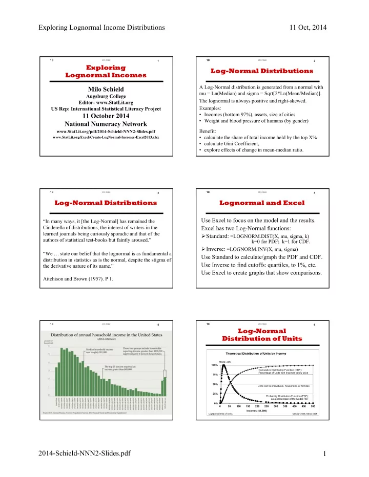
Log-Normal Distribution of Units
0% 25% 50% 75% 100% 50 100 150 200 250 300 350 400 450 500 Incomes ($1,000)
Theoretical Distribution of Units by Income
Probability Distribution Function (PDF): as a percentage of the Modal PDF Cumulative Distribution Function (CDF): Percentage of Units with Incomes below price Mode: 20K LogNormal Dist of Units Median=50K; Mean=80K Units can be individuals, households or families