Lecture 5: Probability Distributions Random Variables - PDF document

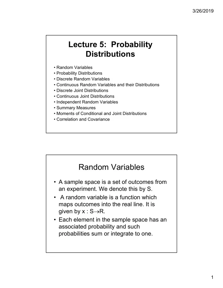
3/26/2019 Lecture 5: Probability Distributions • Random Variables • Probability Distributions • Discrete Random Variables • Continuous Random Variables and their Distributions • Discrete Joint Distributions • Continuous Joint Distributions • Independent Random Variables • Summary Measures • Moments of Conditional and Joint Distributions • Correlation and Covariance Random Variables • A sample space is a set of outcomes from an experiment. We denote this by S. • A random variable is a function which maps outcomes into the real line. It is given by x : S  R. • Each element in the sample space has an associated probability and such probabilities sum or integrate to one. 1

3/26/2019 Probability Distributions • Let A  R and let Prob(x  A) denote the probability that x will belong to A. • Def . The distribution function of a random variable x is a function defined by F(x')  Prob(x  x'), x'  R. Key Properties P.1 F is nondecreasing in x. P.2 lim x  F(x) = 1 and lim x  F(x) = 0. P.3 F is continuous from the right. P.4 For all x', Prob(x > x') = 1 - F(x'). 2

3/26/2019 Discrete Random Variables • If the random variable can assume only a finite number or a countable infinite set of values, it is said to be a discrete random variable. Key Properties P.1 Prob(x = x')  f(x')  0. (f is called the probability mass function or the probability function .)        P.2 f x ( ) Pr ob x ( x ) 1. i i i  1 i  1 P.3 Prob(x  A) =  f x i ( ).  x A i 3

3/26/2019 Examples Example: #1 Consider the random variable associated with 2 tosses of a fair coin. The possible values for the #heads x are {0, 1, 2}. We have that f(0) = 1/4, f(1) = 1/2, and f(2) = 1/4. f(x) F(x) 1 X 1/2 X 3/4 X 1/4 X X 1/4 X 0 1 2 0 1 2 Examples #2 A single toss of a fair die. f(x) = 1/6 if x i = 1,2,3,4,5,6. F(x i ) = x i /6. 4

3/26/2019 Continuous Random Variables and their Distributions Def . A random variable x has a continuous distribution if there exists a nonnegative function f defined on R such that for any interval A of R Prob (x  A) = f x dx ( ) .  x A  The function f is called the probability density function of x and the domain of f is called the support of the random variable x. Properties of f P.1 f(x)  0, for all x.   1 P.2 f x dx ( ) .   P.3 If dF/dx exists, then dF/dx = f(x), for all x. In terms of geometry F(x) is the area under f(x) for x'  x. 5

3/26/2019 Example Example: The uniform distribution on [a,b].  1/(b-a), if x  [a,b] f(x) =   0, otherwise Note that F is given by  1 a 1 x    x   F(x) = [ / ( 1 b a dx )] a x | a x . a    ( b ) ( b a ) ( b ) a Also,  1 a b b ( ) b f x dx  [ / ( 1 b  a dx )]  x | b    1 .   a a    ( b a ) ( b a ) ( b a ) a Example F(x) 1 slope =1/(b-a) -a/(b-a) a b x f(x) 1/(b-a) a b x 6

3/26/2019 Discrete Joint Distributions • Let the two random variables x and y have a joint probability function f(x i ', , y i ') = Prob(x i = x i ' and y i = y i '). Properties of Prob Function P.1 f(x i , y i )  0. P.2 Prob((x i ,y i )  A) =  f x y ( , ) . i i )  ( x y , A i i  P.3 f x y ( , ) = 1. i i ( x y , ) i i 7

3/26/2019 The Distribution Function Defined ' , y i ' ) = Prob( x i  x i ' and y i  y i ' ) = F(x i  f x y ( , ) , where i i )  ( x y , L i i L = {(x i , y i ) : x i  x i ' and y i  y i ' }. Marginal Prob and Distribution Functions • The marginal probability function associated with x is given by f 1 (x j )   Prob(x = x j ) = f ( x , y ) j i y i • The marginal probability function associated with y is given by f 2 (y j )  Prob(y = y j ) =  f x ( , y ) i j x i 8

3/26/2019 Marginal distribution functions • The marginal distribution function of x is given by F 1 (x j ) = Prob(x i  x j ) = lim y j  Prob(x i  x j and y i  y j ) = lim y j  F(x j ,y j ). • Likewise for y, the marginal distribution function is F 2 (y j ) = lim x j  F(x j ,y j ). Example An example . Let x and y represent random variables representing whether or not two different stocks will increase or decrease in price. Each of x and y can take on the values 0 or 1, where a 1 means that its price has increased and a 0 means that it has decreased. The probability function is described by f(1,1) = .50 f(0,1) = .35 f(1,0) = .10 f(0,0) = .05. Answer each of the following questions. a. Find F(1,0) and F(0,1). F(1,0) = .1 + .05 = .15. F(0,1) = .35 + .05 = .40. b. Find F 1 (0) = lim y  1 F(0,y) = F(0,1) = .4 c. Find F 2 (1) = lim x  1 F(x,1) = F(1,1) = 1. d. Find f 1 (0) =   f(0,1) + f(0,0) = .4. f ( , ) 0 y y   e. Find f 1 (1) = f ( , ) 1 y f(1,1) +f(1,0) =.6 y 9

3/26/2019 Conditional Distributions • After a value of y has been observed, the probability that a value of x will be observed is given by   Prob(x = x i | y = y i ) = Pr ob x ( x & y y ) i i .  Pr ob y ( y ) i • The function g 1 (x i | y i )  f x y ( , ) i i ( ) . f y 2 i is called the conditional probability function of x , given y. g 2 (y i | x i ) is defined analogously. Properties of Conditional Probability Functions (i) g 1 (x i | y i )  0.  g 1 (x i | y i ) =  f(x i ,y i ) /  f(x i ,y i ) = 1. (ii) x i x i x i ((i) and (ii) hold for g 2 (y i | x i )) (iii) f(x i ,y i ) = g 1 (x i | y i )f 2 (y i ) = g 2 (y i | x i )f 1 (x i ). 10

3/26/2019 Conditional Distribution Functions F 1 (x i | y i ) =  f x y ( , ) / f ( y ) , i i 2 i  x x i  F 2 (y i | x i ) = f x y ( , ) / f x ( ) . i i 1 i  y y i The stock price example revisited a. Compute g 1 (1 | 0) = f(1,0)/f 2 (0). We have that f 2 (0) = f(0,0) + f(1,0) = .05 + .1 = .15. Further f(1,0) = .1. Thus, g 1 (1 | 0) = .1/.15 = .66.  b. Find g 2 (0 | 0) = f(0,0)/f 1 (0) = .05/.4 = .125. Here f 1 (0) = f ( , 0 y i ) = f(0,0) + f(0,1) = .05 + .35 y i = .4. 11

3/26/2019 Continuous Joint Distributions • The random variables x and y have a continuous joint distribution if there exists a nonnegative function f defined on R 2 such that for any A  R 2 Prob((x,y)  A) =  f x y dxdy ( , ) . A • f is called the joint probability density function of x and y. Properties of f • f satisfies the usual properties: P.1 f(x,y)  0.   P.2 f(x,y)dxdy = 1.     12

3/26/2019 Distribution function y' x' F(x',y') = Prob(x  x' and y  y') = f(x,y)dxdy.     If F is tw i c e d if fe re nt ia b le , th e n w e h a ve t ha t f(x ,y) =  2 F ( x,y )/  x  y . Marginal Density and Distribution Functions • The marginal density and distribution functions are defined as follows: a. F 1 (x) = lim y  F(x,y) and F 2 (y) = lim x  F(x,y). (marginal distribution functions) b. f 1 (x) = f x y ( , ) dy and f 2 (y) = f x y  ( , ) dx.  y x 13

3/26/2019 Example Let f(x,y) = 4xy for x,y  [0,1] and 0 otherwise. 1 1 a. Check to see that 4xydxdy = 1.   0 0 y ' x ' xydxdy = (x') 2 (y') 2 . Note also that  2 F/  x  y = 4xy = b. Find F(x',y'). Clearly, F(x',y') = 4   0 0 f(x,y). c. Find F 1 (x) and F 2 (y). We have that 2 = x 2 . 2 F 1 (x) = lim x y  1 y Using similar reasoning, F 2 (y) = y 2 . d. Find f 1 (x) and f 2 (y). 1 1 f 1 (x) = f(x,y)dy = 2x and f 2 (y) = f(x,y)dx = 2y.   0 0 Conditional Density • We have The conditional density function of x, given that y is fixed at a particular value is given by g 1 (x | y) = f(x,y)/f 2 (y). Likewise, for y we have g 2 (y | x) = f(x,y)/f 1 (x). It is clear that  g 1 (x | y)dx = 1. 14

3/26/2019 Conditional Distribution Functions • We have The conditional distribution functions are given by x' G 1 (x' | y) =  g 1 (x |y)dx,  y' G 2 (y' | x) = g 2 (y |x)dy.   Example : Let us revisit example #2 above. We have that f = 4xy with x,y  (0,1). g 1 (x | y) = 4xy/2y = 2x and g 2 (y | x) = 4xy/2x = 2y. Moreover, x 2  x dx = 2 ( ') x' = (x') 2 . G 1 (x' | y) = 2 2 0 By symmetry. G 2 (y’ | x) = (y') 2 . It turns out that in this example, x and y are independent random variables, because the conditional distributions do not depend on the other random variable. 15