Formal Modeling in Cognitive Science 1 Distributions Lecture 20: - PowerPoint PPT Presentation

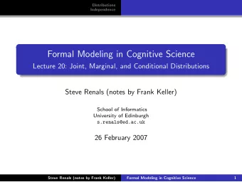
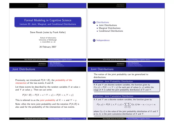
Distributions Distributions Independence Independence Formal Modeling in Cognitive Science 1 Distributions Lecture 20: Joint, Marginal, and Conditional Distributions Joint Distributions Marginal Distributions Conditional Distributions Steve Renals (notes by Frank Keller) School of Informatics University of Edinburgh 2 Independence s.renals@ed.ac.uk 26 February 2007 Steve Renals (notes by Frank Keller) Formal Modeling in Cognitive Science 1 Steve Renals (notes by Frank Keller) Formal Modeling in Cognitive Science 2 Joint Distributions Joint Distributions Distributions Distributions Marginal Distributions Marginal Distributions Independence Independence Conditional Distributions Conditional Distributions Joint Distributions Joint Distributions The notion of the joint probability can be generalized to distributions: Previously, we introduced P ( A ∩ B ), the probability of the Definition: Joint Probability Distribution intersection of the two events A and B . If X and Y are discrete random variables, the function given by Let these events be described by the random variables X at value x f ( x , y ) = P ( X = x , Y = y ) for each pair of values ( x , y ) within the and Y at value y . Then we can write: range of X is called the joint probability distribution of X and Y . P ( A ∩ B ) = P ( X = x ∩ Y = y ) = P ( X = x , Y = y ) Definition: Joint Cumulative Distribution If X and Y are a discrete random variables, the function given by: This is referred to as the joint probability of X = x and Y = y . Note: often the term joint probability and the notation P ( A , B ) is � � F ( x , y ) = P ( X ≤ x , Y ≤ y ) = f ( s , t ) for − ∞ < x , y < ∞ also used for the probability of the intersection of two events. s ≤ x t ≤ y where f ( s , t ) is the value of the joint probability distribution of X and Y at ( s , t ), is the joint cumulative distribution of X and Y . Steve Renals (notes by Frank Keller) Formal Modeling in Cognitive Science 3 Steve Renals (notes by Frank Keller) Formal Modeling in Cognitive Science 4

Joint Distributions Joint Distributions Distributions Distributions Marginal Distributions Marginal Distributions Independence Independence Conditional Distributions Conditional Distributions Example: Corpus Data Example: Corpus Data Assume you have a corpus of a 100 words (a corpus is a collection of text; see Informatics 1B). You tabulate the words, their We can now define the following random variables: frequencies and probabilities in the corpus: X : the length of the word; Y : number of vowels in the word. c ( w ) P ( w ) w x y the 30 0.30 3 1 Examples for probability distributions: to 18 0.18 2 1 will 16 0.16 4 1 f X (5) = P (Earth) + P (probe) + P (Comet) = 0 . 14; of 10 0.10 2 1 f Y (2) = P (Earth) + P (probe) + P (some) + P (Comet) = 0 . 17. Earth 7 0.07 5 2 on 6 0.06 2 1 Examples for cumulative distributions: probe 4 0.04 5 2 F X (3) = f X (2) + f X (3) = 0 . 34 + 0 . 33 = 0 . 67; some 3 0.03 4 2 Comet 3 0.03 5 2 F Y (1) = f X (0) + f X (1) = 0 . 03 + 0 . 80 = 0 . 83. BBC 3 0.03 3 0 Steve Renals (notes by Frank Keller) Formal Modeling in Cognitive Science 5 Steve Renals (notes by Frank Keller) Formal Modeling in Cognitive Science 6 Joint Distributions Joint Distributions Distributions Distributions Marginal Distributions Marginal Distributions Independence Independence Conditional Distributions Conditional Distributions Example: Corpus Data Marginal Distributions Now compute the joint distribution of X and Y as f ( x , y ) = P ( X = x , Y = y ). If we ‘project’ one of the two dimensions of a joint distributions, Examples: we obtain a marginal distributions: f (2 , 1) = P (to) + P (of) + P (on) = 0 . 18 + 0 . 10 + 0 . 06 = 0 . 34; Definition: Marginal Distribution f (3 , 0) = P (BBC) = 0 . 03; If X and Y are discrete random variables and f ( x , y ) is the value of f (4 , 3) = 0. their joint probability distribution at ( x , y ), the functions given by: Full distribution: � � g ( x ) = f ( x , y ) and h ( y ) = f ( x , y ) x y x 2 3 4 5 are the marginal distributions of X and Y , respectively. 0 0 0.03 0 0 y 1 0.34 0.30 0.16 0 2 0 0 0.03 0.14 Steve Renals (notes by Frank Keller) Formal Modeling in Cognitive Science 7 Steve Renals (notes by Frank Keller) Formal Modeling in Cognitive Science 8

Joint Distributions Joint Distributions Distributions Distributions Marginal Distributions Marginal Distributions Independence Independence Conditional Distributions Conditional Distributions Example: Corpus Data Conditional Distributions We had defined the following random variables: Previously, we defined the conditional probability of two events A X : the length of the word; and B as follows: Y : number of vowels in the word. P ( B | A ) = P ( A ∩ B ) P ( A ) Joint distribution of X and Y : Let these events be described by the random variable X = x and x Y = y . Then we can write: 2 3 4 5 � x f ( x , y ) P ( X = x | Y = y ) = P ( X = x , Y = y ) = f ( x , y ) 0 0 0.03 0 0 0.03 P ( Y = y ) h ( y ) y 1 0.34 0.30 0.16 0 0.80 2 0 0 0.03 0.14 0.17 where f ( x , y ) is the joint probability distribution of X and Y and � y f ( x , y ) 0.34 0.33 0.19 0.14 h ( y ) is the marginal marginal distribution of y . Marginal distribution of Y . Marginal distribution of X. Steve Renals (notes by Frank Keller) Formal Modeling in Cognitive Science 9 Steve Renals (notes by Frank Keller) Formal Modeling in Cognitive Science 10 Joint Distributions Joint Distributions Distributions Distributions Marginal Distributions Marginal Distributions Independence Independence Conditional Distributions Conditional Distributions Conditional Distributions Example: Corpus Data Definition: Conditional Distribution Based on the joint distribution f ( x , y ) and the marginal If f ( x , y ) is the value of the joint probability distribution of the distributions h ( y ) and g ( x ) from the previous example, we can discrete random variables X and Y at ( x , y ) and h ( y ) is the value compute the conditional distributions of X given Y = 1: of the marginal distributions of Y at y , and g ( x ) is the value of the marginal distributions of X at x , then: x 2 3 4 5 f ( x | y ) = f ( x , y ) w ( y | x ) = f ( x , y ) f (2 , 1) f (3 , 1) f (4 , 1) f (5 , 1) h (1) = h (1) = h (1) = h (1) = and h ( y ) g ( x ) 0 . 34 0 . 30 0 . 16 0 y 1 0 . 80 = 0 . 80 = 0 . 80 = 0 . 80 = 0.43 0.38 0.20 0 are the conditional distributions of X given Y = y , and of Y given X = x , respectively (for h ( y ) � = 0 and g ( x ) � = 0). Steve Renals (notes by Frank Keller) Formal Modeling in Cognitive Science 11 Steve Renals (notes by Frank Keller) Formal Modeling in Cognitive Science 12

Distributions Distributions Independence Independence Independence Example: Corpus Data Marginal distributions from the previous example: The notion of independence of events can also be generalized to x probability distributions: 2 3 4 5 h ( y ) Definition: Independence 0 0 0.03 0 0 0.03 1 0.34 0.30 0.16 0 0.80 y If f ( x , y ) is the value of the joint probability distribution of the 2 0 0 0.03 0.14 0.17 discrete random variables X and Y at ( x , y ), and g ( x ) and h ( y ) g ( x ) 0.34 0.33 0.19 0.14 are the values of the marginal distributions of X at x and Y at y , respectively, then X and Y are independent iff: Now compute g ( x ) h ( y ) for each cell in the table: f ( x , y ) = g ( x ) h ( y ) x 2 3 4 5 for all ( x , y ) within their range. X and Y are 0 0.01 0.01 0.01 0.00 not independent. 1 0.27 0.26 0.15 0.12 y 2 0.06 0.06 0.03 0.02 Steve Renals (notes by Frank Keller) Formal Modeling in Cognitive Science 13 Steve Renals (notes by Frank Keller) Formal Modeling in Cognitive Science 14 Distributions Independence Summary A joint probability distribution returns a probability for each pair of values of two random variables. marginal distributions project one of the dimensions of a joint probability distribution; the conditional distribution is the joint distribution divided by the marginal distribution; two distributions are independent if the joint distribution is the same as the product of the two marginal distributions. Steve Renals (notes by Frank Keller) Formal Modeling in Cognitive Science 15