Probability Density (1) Let f ( x 1 , x 2 . . . x n ) be a - PDF document

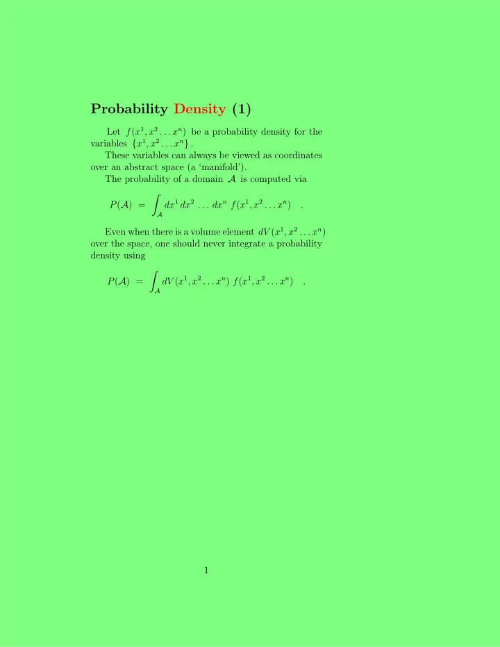
Probability Density (1) Let f ( x 1 , x 2 . . . x n ) be a probability density for the variables { x 1 , x 2 . . . x n } . These variables can always be viewed as coordinates over an abstract space (a ‘manifold’). The probability of a domain A is computed via � dx 1 dx 2 . . . dx n f ( x 1 , x 2 . . . x n ) P ( A ) = . A Even when there is a volume element dV ( x 1 , x 2 . . . x n ) over the space, one should never integrate a probability density using � dV ( x 1 , x 2 . . . x n ) f ( x 1 , x 2 . . . x n ) P ( A ) = . A 1

Probability Density (2) When changing from the variables { x 1 , x 2 . . . x n } to some other variables { y 1 , y 2 . . . y n } , the probability dis- tribution that was represented by the probability den- sity f ( x 1 , x 2 . . . x n ) is now represented by a probability density g ( y 1 , y 2 . . . y n ) , and one has (Jacobian rule) g ( y 1 , y 2 . . . y n ) = f ( x 1 , x 2 . . . x n ) J , where J is the absolute value of the determinant of the matrix of partial derivatives ∂x 1 ∂x 1   · · · ∂y 1 ∂y n . . ... . . .   . .   ∂x n ∂x n · · · ∂y 1 ∂y n 2

Marginal Probability Density When the whole set of variables { x 1 , x 2 . . . x n } naturally separates into two groups of variables { u 1 , u 2 . . . u p } and { v 1 , v 2 . . . v q } (with p + q = n ), all the information con- cerning the variables { u 1 , u 2 . . . u p } alone is contained in the marginal probability density f u ( u 1 , u 2 . . . u p ) = � dv 1 . . . dv q f ( u 1 , u 2 . . . u p , v 1 , v 2 . . . v q ) = . all range Similarly, all the information concerning the variables { v 1 , v 2 . . . v q } alone is contained in the marginal proba- bility density f v ( v 1 , v 2 . . . v q ) = � du 1 . . . du p f ( u 1 , u 2 . . . u p , v 1 , v 2 . . . v q ) = . all range 3

Warning This definition of marginal probability density is, ex- cepted for some minor interpretation details, safe. The same is not true for the definition of conditional probability density . The simple definition one finds in most texts is usually overinterpreted, and leads to para- doxes, the most famous of all being the ‘Borel paradox’. 4

Reproduced from Kolmogorov’s Foundations of the The- ory of Probability (1950, pp. 50–51). § 2. Explanation of a Borel Paradox Let us choose for our basic set E the set of all points on a spherical surface. Our F will be the aggregate of all Borel sets of the spherical surface. And finally, our P ( A ) is to be proportional to the measure set of A . Let us now choose two diametrically opposite points for our poles, so that each meridian circle will be uniquely defined by the longitude ψ , 0 ≤ ψ < π . Since ψ varies from 0 only to π , — in other words, we are considering complete meridian circles (and not merely semicircles) — the latitude θ must vary from − π to + π (and not from − π 2 to + π 2 ). Borel set the following problem: Required to determine “the conditional probability distribution” of latitude θ , − π ≤ θ < + π , for a given longitude ψ . It is easy to calculate that � θ 2 P ψ ( θ 1 ≤ θ < θ 2 ) = 1 | cos θ | dθ . 4 θ 1 The probability distribution of θ for a given ψ is not uniform. If we assume the the conditional probability distri- bution of θ “with the hypothesis that ξ lies on the given meridian circle” must be uniform, then we have arrived at a contradiction. This shows that the concept of a conditional proba- bility with regard to an isolated given hypothesis whose probability equals 0 is inadmissible. For we van obtain a probability distribution for θ on the meridian circle only if we regard this circle as an element of the decomposi- tion of the entire spherical surface into meridian circles with the given poles. 5

Conditional Probability (Not yet conditional probability density ) P ( A|B ) = P ( A ∩ B ) P ( B ) 6

f ( u, v 0 ) f ( u | v 0 ) = � du f ( u, v 0 ) 7

f ( u , v ( u ) ) f ( u | v = v ( u ) ) = � du f ( u , v ( u ) ) 8

The Borel Paradox an example of the danger of overinter- preting the usual definition of conditional probability density Arbitrary probability density over the sphere, using spher- ical coordinates: f ( θ, ϕ ) . �� P ( A ) = dθ dϕ f ( θ, ϕ ) A The homogeneous probability density: � π � 2 π f ( θ, ϕ ) = sin θ ; dϕ f ( θ, ϕ ) = 1 dθ 4 π 0 0 9

Marginal probability density for θ : � 2 π dϕ f ( θ, ϕ ) = sin θ f θ ( θ ) = 2 0 Marginal probability density for ϕ : � π 1 f ϕ ( ϕ ) = dθ f ( θ, ϕ ) = 2 π 0 → interpretation O.K. 10

A point P has materialized on the surface of the sphere, with homogeneous probability density, and we are told that it has materialized in the meridian defined by ϕ = ϕ 0 . Which is the probability density for the colatitude θ ? Conditional probability density for θ given ϕ = ϕ 0 : 0 dθ f ( θ, ϕ 0 ) = sin θ f ( θ, ϕ 0 ) f θ | ϕ ( θ | ϕ = ϕ 0 ) = � π 2 11

Rather than developing here the theory that is totally free from those inconsistencies (and to propose more general formulas for the conditional probability density), I choose to take the formulas above as they are, and give (later on) the precise conditions for their validity. (conditions that are not fulfilled in the Borel problem. . . ) 12

Bayes’ Theorem Some variables { u , v } = { u 1 , u 2 , . . . , v 1 , v 2 , . . . } ‘Joint’ probability density: f ( u , v ) � Marginal probability density: f v ( v ) = d u f ( u , v ) f ( u , v 0 ) Conditional probability density: f ( u | v 0 ) = R d u f ( u , v 0 ) f ( u , v ) f ( u | v ) = R d u f ( u , v ) Using the definition of marginal probability density, the conditional probability density can be written f ( u | v ) = f ( u , v ) f v ( v ) Therefore, f ( u , v ) = f ( u | v ) f v ( v ) 13