Lecture 15: More Probability. Summary. CS70: Onwards. Events, - - PowerPoint PPT Presentation

Lecture 15: More Probability.

Events, Conditional Probability, Independence, Bayes’ Rule

Summary.

Modeling Uncertainty: Probability Space

• 1. Random Experiment
• 2. Probability Space: Ω;Pr[ω] ∈ [0,1];∑ω Pr[ω] = 1.
• 3. Uniform Probability Space: Pr[ω] = 1/|Ω| for all ω ∈ Ω.
• 4. Event: “subset of outcomes.” A ⊆ Ω. Pr[A] = ∑w∈A Pr[ω]
• 5. Some calculations.

CS70: Onwards.

Events, Conditional Probability, Independence, Bayes’ Rule

• 1. Probability Basics Review
• 2. Events
• 3. Conditional Probability
• 4. Independence of Events
• 5. Bayes’ Rule

Probability Basics Review

Setup:

◮ Random Experiment.

Flip a fair coin twice.

◮ Probability Space.

◮ Sample Space: Set of outcomes, Ω.

Ω = {HH,HT,TH,TT} (Note: Not Ω = {H,T} with two picks!)

◮ Probability: Pr[ω] for all ω ∈ Ω.

Pr[HH] = ··· = Pr[TT] = 1/4

• 1. 0 ≤ Pr[ω] ≤ 1.
• 2. ∑ω∈Ω Pr[ω] = 1.

Probability: Events.

An event A in a probability space, Ω,Pr[·], is A ⊆ Ω. The probability of an event A is Pr[A] = ∑ωinΩ Pr[ω]. Don’t sweat Pr[A] or Pr(A). Same deal. Examples: Flip two coins: Event A - exactly one heads. Ω = {HH,HT,TH,TT}. A = {HT,TH}. Deal a poker head: Event four aces. Ω = all five card poker hands. |Ω| = 52

5

• A = the poker hands with four aces. |A| = 48.

Flip 2n coins: Event A - exactly n heads. Ω = {H,T}2n. |Ω| = 22n A is set of outcomes with n heads. |A| = 2n

n

• .

Approximation: roughly 1/√πn. = ⇒ not surprising to have something like n +√πn/2 heads

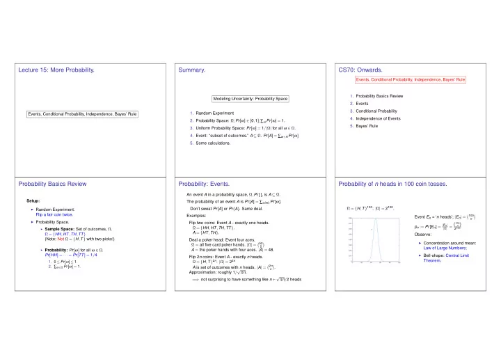
Probability of n heads in 100 coin tosses.

Ω = {H,T}100; |Ω| = 2100.

n p n

Event En = ‘n heads’; |En| = 100

n

• pn := Pr[En] = |En|

|Ω| = (100

n )

2100

Observe:

◮ Concentration around mean:

Law of Large Numbers;

◮ Bell-shape: Central Limit

Theorem.

Probability is Additive

Theorem (a) If events A and B are disjoint, i.e., A∩B = / 0, then Pr[A∪B] = Pr[A]+Pr[B]. (b) If events A1,...,An are pairwise disjoint, i.e., Ak ∩Am = / 0,∀k = m, then Pr[A1 ∪···∪An] = Pr[A1]+···+Pr[An]. Proof:

• Obvious. Straightforward. Use definition of probability of events.

Consequences of Additivity

Theorem (a) Pr[A∪B] = Pr[A]+Pr[B]−Pr[A∩B]; (inclusion-exclusion property) (b) Pr[A1 ∪···∪An] ≤ Pr[A1]+···+Pr[An]; (union bound) (c) If A1,...AN are a partition of Ω, i.e., pairwise disjoint and ∪N

m=1Am = Ω, then

Pr[B] = Pr[B ∩A1]+···+Pr[B ∩AN]. (law of total probability) Proof: (b) is obvious. Doh! Add probabilities of outcomes once on LHS and at least once on RHS. Proofs for (a) and (c)? Next...

Inclusion/Exclusion

Pr[A∪B] = Pr[A]+Pr[B]−Pr[A∩B] Another view. Any ω ∈ A∪B is in A∩B, A∪B, or A∩B. So, add it up.

Total probability

Assume that Ω is the union of the disjoint sets A1,...,AN. Then, Pr[B] = Pr[A1 ∩B]+···+Pr[AN ∩B]. Indeed, B is the union of the disjoint sets An ∩B for n = 1,...,N. In “math”: ω ∈ B is in exactly one of Ai ∩B. Adding up probability of them, get Pr[ω] in sum. ..Did I say... Add it up.

Roll a Red and a Blue Die.

E1 = ‘Red die shows 6’;E2 = ‘Blue die shows 6’ E1 ∪E2 = ‘At least one die shows 6’ Pr[E1] = 6 36,Pr[E2] = 6 36,Pr[E1 ∪E2] = 11 36.

Conditional probability: example.

Two coin flips. First flip is heads. Probability of two heads? Ω = {HH,HT,TH,TT}; Uniform probability space. Event A = first flip is heads: A = {HH,HT}. New sample space: A; uniform still. Event B = two heads. The probability of two heads if the first flip is heads. The probability of B given A is 1/2.

A similar example.

Two coin flips. At least one of the flips is heads. → Probability of two heads? Ω = {HH,HT,TH,TT}; uniform. Event A = at least one flip is heads. A = {HH,HT,TH}. New sample space: A; uniform still. Event B = two heads. The probability of two heads if at least one flip is heads. The probability of B given A is 1/3.

Conditional Probability: A non-uniform example

Red Green Yellow Blue

Ω

3/10 4/10 2/10 1/10

P r [ω ]

Physical experiment Probability model Ω = {Red, Green, Yellow, Blue} Pr[Red|Red or Green] = 3 7 = Pr[Red∩(Red or Green)] Pr[Red or Green]

Another non-uniform example

Consider Ω = {1,2,...,N} with Pr[n] = pn. Let A = {3,4},B = {1,2,3}. Pr[A|B] = p3 p1 +p2 +p3 = Pr[A∩B] Pr[B] .

Yet another non-uniform example

Consider Ω = {1,2,...,N} with Pr[n] = pn. Let A = {2,3,4},B = {1,2,3}. Pr[A|B] = p2 +p3 p1 +p2 +p3 = Pr[A∩B] Pr[B] .

Conditional Probability.

Definition: The conditional probability of B given A is Pr[B|A] = Pr[A∩B] Pr[A] A B A B In A! In B? Must be in A∩B. A∩B Pr[B|A] = Pr[A∩B]

Pr[A] .

More fun with conditional probability.

Toss a red and a blue die, sum is 4, What is probability that red is 1? Pr[B|A] = |B∩A|

|A|

= 1

3; versus Pr[B] = 1/6.

B is more likely given A.

Yet more fun with conditional probability.

Toss a red and a blue die, sum is 7, what is probability that red is 1? Pr[B|A] = |B∩A|

|A|

= 1

6; versus Pr[B] = 1 6.

Observing A does not change your mind about the likelihood of B.

Emptiness..

Suppose I toss 3 balls into 3 bins. A =“1st bin empty”; B =“2nd bin empty.” What is Pr[A|B]? Pr[B] = Pr[{(a,b,c) | a,b,c ∈ {1,3}] = Pr[{1,3}3] = 8

27

Pr[A∩B] = Pr[(3,3,3)] = 1

27

Pr[A|B] = Pr[A∩B]

Pr[B]

= (1/27)

(8/27) = 1/8; vs. Pr[A] = 8 27.

A is less likely given B: Second bin is empty = ⇒ first bin is more likely to contain ball(s).

Gambler’s fallacy.

Flip a fair coin 51 times. A = “first 50 flips are heads” B = “the 51st is heads” Pr[B|A] ? A = {HH ···HT,HH ···HH} B ∩A = {HH ···HH} Uniform probability space. Pr[B|A] = |B∩A|

|A|

= 1

2.

Same as Pr[B]. The likelihood of 51st heads does not depend on the previous flips.

Product Rule

Recall the definition of conditional probability: Pr[B|A] = Pr[A∩B] Pr[A] . Hence, Pr[A∩B] = Pr[A]Pr[B|A]. Consequently, Pr[A∩B ∩C] = Pr[(A∩B)∩C] = Pr[A∩B]Pr[C|A∩B] = Pr[A]Pr[B|A]Pr[C|A∩B].

Product Rule

Theorem Product Rule Let A1,A2,...,An be events. Then Pr[A1 ∩···∩An] = Pr[A1]Pr[A2|A1]···Pr[An|A1 ∩···∩An−1]. Proof: By induction. Assume the result is true for n. (It holds for n = 2.) Then, Pr[A1 ∩···∩An ∩An+1] = Pr[A1 ∩···∩An]Pr[An+1|A1 ∩···∩An] = Pr[A1]Pr[A2|A1]···Pr[An|A1 ∩···∩An−1]Pr[An+1|A1 ∩···∩An],

Thus, the result holds for n +1.

Correlation

An example. Random experiment: Pick a person at random. Event A: the person has lung cancer. Event B: the person is a heavy smoker. Fact: Pr[A|B] = 1.17×Pr[A]. Conclusion:

◮ Smoking increases the probability of lung cancer by 17%. ◮ Smoking causes lung cancer.

Correlation

Event A: the person has lung cancer. Event B: the person is a heavy smoker. Pr[A|B] = 1.17×Pr[A]. A second look. Note that Pr[A|B] = 1.17×Pr[A] ⇔ Pr[A∩B] Pr[B] = 1.17×Pr[A] ⇔ Pr[A∩B] = 1.17×Pr[A]Pr[B] ⇔ Pr[A∩B] Pr[A] = 1.17×Pr[B]. ⇔ Pr[B|A] = 1.17×Pr[B]. Conclusion:

◮ Lung cancer increases the probability of smoking by 17%. ◮ Lung cancer causes smoking. Really?

Causality vs. Correlation

Events A and B are positively correlated if Pr[A∩B] > Pr[A]Pr[B]. (E.g., smoking and lung cancer.) A and B being positively correlated does not mean that A causes B or that B causes A. Other examples:

◮ Tesla owners are more likely to be rich. That does not mean that

poor people should buy a Tesla to get rich.

◮ People who go to the opera are more likely to have a good

• career. That does not mean that going to the opera will improve

your career.

◮ Rabbits eat more carrots and do not wear glasses. Are carrots

good for eyesight?

Proving Causality

Proving causality is generally difficult. One has to eliminate external causes of correlation and be able to test the cause/effect relationship (e.g., randomized clinical trials). Some difficulties:

◮ A and B may be positively correlated because they have a

common cause. (E.g., being a rabbit.)

◮ If B precedes A, then B is more likely to be the cause. (E.g.,

smoking.) However, they could have a common cause that induces B before A. (E.g., studious, CS70, Tesla.) More about such questions later. For fun, check “N. Taleb: Fooled by randomness.”

Total probability

Assume that Ω is the union of the disjoint sets A1,...,AN. Then, Pr[B] = Pr[A1 ∩B]+···+Pr[AN ∩B]. Indeed, B is the union of the disjoint sets An ∩B for n = 1,...,N. Thus, Pr[B] = Pr[A1]Pr[B|A1]+···+Pr[AN]Pr[B|AN].

Total probability

Assume that Ω is the union of the disjoint sets A1,...,AN. Pr[B] = Pr[A1]Pr[B|A1]+···+Pr[AN]Pr[B|AN].

Is you coin loaded?

Your coin is fair (Pr[H] = 0.5) w/prob 1/2 or ’unfair’ (Pr[H] = 0.6),

• therwise.

You flip your coin and it yields heads. What is the probability that it is fair? Analysis: A = ‘coin is fair’,B = ‘outcome is heads’ We want to calculate P[A|B]. We know P[B|A] = 1/2,P[B|¯ A] = 0.6,Pr[A] = 1/2 = Pr[¯ A] Now, Pr[B] = Pr[A∩B]+Pr[¯ A∩B] = Pr[A]Pr[B|A]+Pr[¯ A]Pr[B|¯ A] = (1/2)(1/2)+(1/2)0.6 = 0.55. Thus, Pr[A|B] = Pr[A]Pr[B|A] Pr[B] = (1/2)(1/2) (1/2)(1/2)+(1/2)0.6 ≈ 0.45.

Is you coin loaded?

A picture: Imagine 100 situations, among which m := 100(1/2)(1/2) are such that A and B occur and n := 100(1/2)(0.6) are such that ¯ A and B occur. Thus, among the m +n situations where B occurred, there are m where A occurred. Hence, Pr[A|B] = m m +n = (1/2)(1/2) (1/2)(1/2)+(1/2)0.6.

Independence

Definition: Two events A and B are independent if Pr[A∩B] = Pr[A]Pr[B]. Examples:

◮ When rolling two dice, A = sum is 7 and B = red die is 1 are

independent; Pr[A∩B] = 1

36, Pr[A]Pr[B] =

1

6

1

6

• .

◮ When rolling two dice, A = sum is 3 and B = red die is 1 are not

independent; Pr[A∩B] = 1

36, Pr[A]Pr[B] =

2

36

1

6

• .

◮ When flipping coins, A = coin 1 yields heads and B = coin 2

yields tails are independent; Pr[A∩B] = 1

4, Pr[A]Pr[B] =

1

2

1

2

• .

◮ When throwing 3 balls into 3 bins, A = bin 1 is empty and B =

bin 2 is empty are not independent; Pr[A∩B] = 1

27, Pr[A]Pr[B] =

8

27

8

27

• .

Independence and conditional probability

Fact: Two events A and B are independent if and only if Pr[A|B] = Pr[A]. Indeed: Pr[A|B] = Pr[A∩B]

Pr[B] , so that

Pr[A|B] = Pr[A] ⇔ Pr[A∩B] Pr[B] = Pr[A] ⇔ Pr[A∩B] = Pr[A]Pr[B].

Bayes Rule

Another picture: We imagine that there are N possible causes A1,...,AN. Imagine 100 situations, among which 100pnqn are such that An and B occur, for n = 1,...,N. Thus, among the 100∑m pmqm situations where B occurred, there are 100pnqn where An occurred. Hence, Pr[An|B] = pnqn ∑m pmqm .

Why do you have a fever?

Using Bayes’ rule, we find Pr[Flu|High Fever] = 0.15×0.80 0.15×0.80+10−8 ×1+0.85×0.1 ≈ 0.58 Pr[Ebola|High Fever] = 10−8 ×1 0.15×0.80+10−8 ×1+0.85×0.1 ≈ 5×10−8 Pr[Other|High Fever] = 0.85×0.1 0.15×0.80+10−8 ×1+0.85×0.1 ≈ 0.42 These are the posterior probabilities. One says that ‘Flu’ is the Most Likely a Posteriori (MAP) cause of the high fever.

Bayes’ Rule Operations

Bayes’ Rule is the canonical example of how information changes our

• pinions.

Thomas Bayes

Source: Wikipedia.

Thomas Bayes

A Bayesian picture of Thomas Bayes.

Testing for disease.

Let’s watch TV!! Random Experiment: Pick a random male. Outcomes: (test,disease) A - prostate cancer. B - positive PSA test.

◮ Pr[A] = 0.0016, (.16 % of the male population is affected.) ◮ Pr[B|A] = 0.80 (80% chance of positive test with disease.) ◮ Pr[B|A] = 0.10 (10% chance of positive test without disease.)

From http://www.cpcn.org/01 psa tests.htm and http://seer.cancer.gov/statfacts/html/prost.html (10/12/2011.) Positive PSA test (B). Do I have disease? Pr[A|B]???

Bayes Rule.

Using Bayes’ rule, we find P[A|B] = 0.0016×0.80 0.0016×0.80+0.9984×0.10 = .013. A 1.3% chance of prostate cancer with a positive PSA test. Surgery anyone? Impotence... Incontinence.. Death.

Summary

Events, Conditional Probability, Independence, Bayes’ Rule Key Ideas:

◮ Conditional Probability:

Pr[A|B] = Pr[A∩B]

Pr[B] ◮ Independence: Pr[A∩B] = Pr[A]Pr[B]. ◮ Bayes’ Rule:

Pr[An|B] = Pr[An]Pr[B|An] ∑m Pr[Am]Pr[B|Am]. Pr[An|B] = posterior probability;Pr[An] = prior probability .

◮ All these are possible:

Pr[A|B] < Pr[A];Pr[A|B] > Pr[A];Pr[A|B] = Pr[A].