CS70: Jean Walrand: Lecture 24. Recall definition: Conditional - - PowerPoint PPT Presentation

CS70: Jean Walrand: Lecture 24.

Changing your mind?

• 1. Bayes Rule.
• 2. Examples.

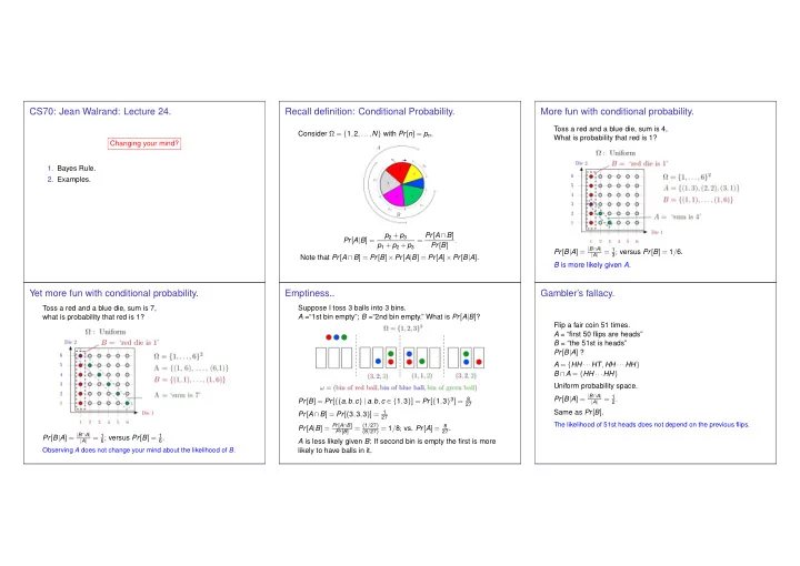
Recall definition: Conditional Probability.

Consider Ω = {1,2,...,N} with Pr[n] = pn. Pr[A|B] = p2 +p3 p1 +p2 +p3 = Pr[A∩B] Pr[B] . Note that Pr[A∩B] = Pr[B]×Pr[A|B] = Pr[A]×Pr[B|A].

More fun with conditional probability.

Toss a red and a blue die, sum is 4, What is probability that red is 1? Pr[B|A] = |B∩A|

|A|

= 1

3; versus Pr[B] = 1/6.

B is more likely given A.

Yet more fun with conditional probability.

Toss a red and a blue die, sum is 7, what is probability that red is 1? Pr[B|A] = |B∩A|

|A|

= 1

6; versus Pr[B] = 1 6.

Observing A does not change your mind about the likelihood of B.

Emptiness..

Suppose I toss 3 balls into 3 bins. A =“1st bin empty”; B =“2nd bin empty.” What is Pr[A|B]? Pr[B] = Pr[{(a,b,c) | a,b,c ∈ {1,3}] = Pr[{1,3}3] = 8

27

Pr[A∩B] = Pr[(3,3,3)] = 1

27

Pr[A|B] = Pr[A∩B]

Pr[B]

= (1/27)

(8/27) = 1/8; vs. Pr[A] = 8 27.

A is less likely given B: If second bin is empty the first is more likely to have balls in it.

Gambler’s fallacy.

Flip a fair coin 51 times. A = “first 50 flips are heads” B = “the 51st is heads” Pr[B|A] ? A = {HH ···HT,HH ···HH} B ∩A = {HH ···HH} Uniform probability space. Pr[B|A] = |B∩A|

|A|

= 1

2.

Same as Pr[B].

The likelihood of 51st heads does not depend on the previous flips.

Monty Hall Game.

Monty Hall is the host of a game show. His assistant is Carol.

◮ Three doors; one prize two goats. ◮ Choose one door, say door 1. ◮ Carol opens another door with a goat, say door 3. ◮ Monty offers you a chance to switch doors, i.e., choose

door 2.

◮ What do you do?

Monty Hall Game

Recall: You picked door 1 and Carol opened door 3. Should you switch to door 2? First intuition: Doors 1 and 2 are equally likely to hide the prize: no need to switch. Opening door 3 did not tell us anything about doors 1 and 2. Wrong! Better observation: If you switch, you get the prize, except it it is behind door 1. Thus, by switching, you get the prize with probability 2/3. If you do not switch, you get it with probability 1/3.

Monty Hall Game Analysis

Ω = {1,2,3}2;ω = (a,b) = ( prize, your initial choice); uniform. If you do not switch, you win if a = b. If you switch, you win if a = b. E.g., (a,b) = (1,2) → shows 3 → switch to 1. Pr[{(a,b) | a = b}] = 3

9 = 1 3

Pr[{(a,b) | a = b}] = 1−Pr[{(a,b) | a = b}] = 2

3.

Independence

Definition: Two events A and B are independent if Pr[A∩B] = Pr[A]Pr[B]. Examples:

◮ When rolling two dice, A = sum is 7 and B = red die is 1

are independent;

◮ When rolling two dice, A = sum is 3 and B = red die is 1

are not independent;

◮ When flipping coins, A = coin 1 yields heads and B = coin

2 yields tails are independent;

◮ When throwing 3 balls into 3 bins, A = bin 1 is empty and

B = bin 2 is empty are not independent;

Independence and conditional probability

Fact: Two events A and B are independent if and only if Pr[A|B] = Pr[A]. Indeed: Pr[A|B] = Pr[A∩B]

Pr[B] , so that

Pr[A|B] = Pr[A] ⇔ Pr[A∩B] Pr[B] = Pr[A] ⇔ Pr[A∩B] = Pr[A]Pr[B].

Total probability

Here is a simple useful fact: Pr[B] = Pr[A∩B]+Pr[¯ A∩B]. Indeed, B is the union of two disjoint sets A∩B and ¯ A∩B. Thus, Pr[B] = Pr[A]Pr[B|A]+Pr[¯ A]Pr[B|¯ A].

Total probability

Assume that Ω is the union of the disjoint sets A1,...,AN. Then, Pr[B] = Pr[A1 ∩B]+···+Pr[AN ∩B]. Indeed, B is the union of the disjoint sets An ∩B for n = 1,...,N. Thus, Pr[B] = Pr[A1]Pr[B|A1]+···+Pr[AN]Pr[B|AN].

Total probability

Assume that Ω is the union of the disjoint sets A1,...,AN. Pr[B] = Pr[A1]Pr[B|A1]+···+Pr[AN]Pr[B|AN].

Is you coin loaded?

Your coin is fair w.p. 1/2 or such that Pr[H] = 0.6, otherwise. You flip your coin and it yields heads. What is the probability that it is fair? Analysis: A = ‘coin is fair’,B = ‘outcome is heads’ We want to calculate P[A|B]. We know P[B|A] = 1/2,P[B|¯ A] = 0.6,Pr[A] = 1/2 = Pr[¯ A] Now, Pr[B] = Pr[A∩B]+Pr[¯ A∩B] = Pr[A]Pr[B|A]+Pr[¯ A]Pr[B|¯ A] = (1/2)(1/2)+(1/2)0.6 = 0.55. Thus, Pr[A|B] = Pr[A]Pr[B|A] Pr[B] = (1/2)(1/2) (1/2)(1/2)+(1/2)0.6 ≈ 0.45.

Is you coin loaded?

A picture: Imagine 100 situations, among which m := 100(1/2)(1/2) are such that A and B occur and n := 100(1/2)(0.6) are such that ¯ A and B occur. Thus, among the m +n situations where B occurred, there are m where A occurred. Hence, Pr[A|B] = m m +n = (1/2)(1/2) (1/2)(1/2)+(1/2)0.6.

Bayes Rule

Another picture: We imagine that there are N possible causes A1,...,AN. Imagine 100 situations, among which 100pnqn are such that An and B occur, for n = 1,...,N. Thus, among the 100∑m pmqm situations where B occurred, there are 100pnqn where An occurred. Hence, Pr[An|B] = pnqn ∑m pmqm .

Why do you have a fever?

Using Bayes’ rule, we find Pr[Flu|High Fever] = 0.15×0.80 0.15×0.80+10−8 ×1+0.85×0.1 ≈ 0.58 Pr[Ebola|High Fever] = 10−8 ×1 0.15×0.80+10−8 ×1+0.85×0.1 ≈ 5×10−8 Pr[Other|High Fever] = 0.85×0.1 0.15×0.80+10−8 ×1+0.85×0.1 ≈ 0.42 These are the posterior probabilities. One says that ‘Flu’ is the Most Likely a Posteriori (MAP) cause of the high fever.

Bayes’ Rule Operations

Bayes’ Rule is the canonical example of how information changes our opinions.

Thomas Bayes

Source: Wikipedia.

Thomas Bayes

A Bayesian picture of Thomas Bayes.

Testing for disease.

Let’s watch TV!! Random Experiment: Pick a random male. Outcomes: (test,disease) A - prostate cancer. B - positive PSA test.

◮ Pr[A] = 0.0016, (.16 % of the male population is affected.) ◮ Pr[B|A] = 0.80 (80% chance of positive test with disease.) ◮ Pr[B|A] = 0.10 (10% chance of positive test without

disease.) From http://www.cpcn.org/01 psa tests.htm and http://seer.cancer.gov/statfacts/html/prost.html (10/12/2011.) Positive PSA test (B). Do I have disease? Pr[A|B]???

Bayes Rule.

Using Bayes’ rule, we find P[A|B] = 0.0016×0.80 0.0016×0.80+0.9984×0.10 = .013. A 1.3% chance of prostate cancer with a positive PSA test. Surgery anyone? Impotence... Incontinence.. Death.

Summary

Change your mind? Key Ideas:

◮ Conditional Probability:

Pr[A|B] = Pr[A∩B] Pr[B]

◮ Bayes’ Rule:

Pr[An|B] = Pr[An]Pr[B|An] ∑m Pr[Am]Pr[B|Am]. Pr[An|B] = posterior probability;Pr[An] = prior probability .

◮ All these are possible:

Pr[A|B] < Pr[A];Pr[A|B] > Pr[A];Pr[A|B] = Pr[A].