Input Distributions Reading: Chapter 6 in Law Input Distributions - - PowerPoint PPT Presentation

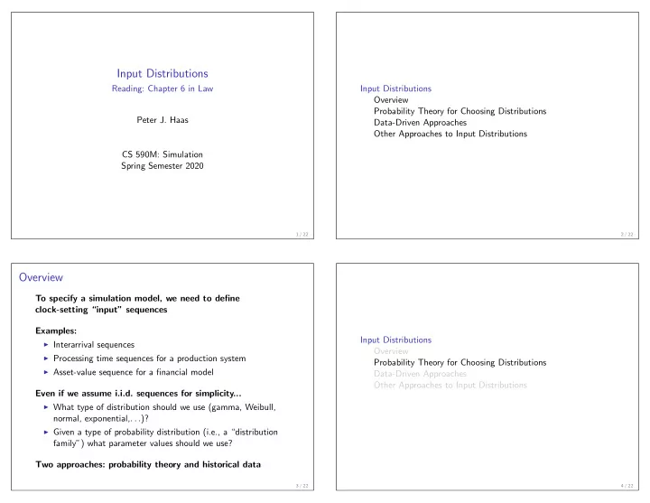
Input Distributions

Reading: Chapter 6 in Law Peter J. Haas CS 590M: Simulation Spring Semester 2020

1 / 22

Input Distributions Overview Probability Theory for Choosing Distributions Data-Driven Approaches Other Approaches to Input Distributions

2 / 22

Overview

To specify a simulation model, we need to define clock-setting “input” sequences Examples:

◮ Interarrival sequences ◮ Processing time sequences for a production system ◮ Asset-value sequence for a financial model

Even if we assume i.i.d. sequences for simplicity...

◮ What type of distribution should we use (gamma, Weibull,

normal, exponential,. . .)?

◮ Given a type of probability distribution (i.e., a “distribution

family”) what parameter values should we use? Two approaches: probability theory and historical data

3 / 22

Input Distributions Overview Probability Theory for Choosing Distributions Data-Driven Approaches Other Approaches to Input Distributions

4 / 22

Theoretical Justification for Normal Random Variables

Suppose that X can be expressed as a sum of random variables: X = Y1 + Y2 + · · · + Yn In great generality, versions of CLT imply that X D ∼ N(µ, σ2) (approx.) for large n, where µ = E[X] and σ2 = Var[X]

◮ Yi’s need not be i.i.d., just not “too dependent” and not “too

non-identical” Q: Examples where CLT breaks down?

Moral:

If X is the sum of a large number of other random quantities, then X can be approx. modeled as a normal random variable.

5 / 22

Theoretical Justification for Lognormal Random Variables

Suppose that X can be expressed as a product of random variables: X = Z1Z2 · · · Zn

◮ Example: Value of a financial asset

Then log(X) = Y1 + Y2 + · · · + Yn, where Yi = log(Zi) By prior discussion, log(X) D ∼ N(µ, σ2) (approx.) for large n, i.e. X D ∼ exp

• N(0, 1)
• , so that X is approximately lognormally

distributed

Moral:

If X is the product of a large number of other random quantities, then X can be approx. modeled as a lognormal random variable.

6 / 22

Theoretical Justification for Poisson Arrival Process

Suppose that the arrival process is a superposition of arrivals from a variety of statistically independent sources

source 1 source 2 source 3 source n : : : queue

The Palm-Khintchine Theorem says that superposition of n i.i.d. sources looks ≈ Poisson as n becomes large

◮ Can relax i.i.d. assumption

Moral:

Poisson process often a reasonable model of arrival processes. (But beware of long-range dependence)

7 / 22

Theoretical Justification for Weibull Distribution

Suppose that X can be expressed as a minimum of nonnegative random variables: X = min1≤i≤n Yi

◮ Example: Lifetime of a complex system

Extreme-value theory (Gnedenko’s Theorem) says that if Yi’s are i.i.d. then X has approximately a Weibull distribution when n is large: P(X ≤ x) = 1 − e−(λx)α

◮ α is the shape parameter and λ is the scale parameter

Moral:

If X is the the lifetime of a complicated component, then X can be

• approx. modeled as a Weibull random variable.

8 / 22

Controlling the Variability

Squared coefficient of variation: ρ2(X) = Var(X) (E[X])2

Case 1: X

D

∼ exp(λ)

ρ2(X) = 1

Case 2: X

D

∼ gamma(λ, α) fX(x) = λe−λx(λx)α−1/Γ(α)

ρ2(X) = α/λ2 (α/λ)2 = 1 α Three scenarios to play with:

◮ α > 1: less variable than exponential ◮ α = 1: exponential ◮ α < 1: more variable than exponential

9 / 22

Input Distributions Overview Probability Theory for Choosing Distributions Data-Driven Approaches Other Approaches to Input Distributions

10 / 22

Goodness-of-Fit Software

GoF software applies a set of goodness-of-fit tests to select distribution family with “best fit” to data

◮ chi-square, Kolmogorov-Smirnov, Epps-Singleton,

Anderson-Darling, . . . GoF software must be used with caution

◮ Low power: Poor discrimination between different distributions ◮ Sequential testing: Test properties mathematically ill-defined ◮ Discourages sensitivity analysis: Unwary users stop with “best” ◮ Can obscure non-i.i.d. features: e.g., trends, autocorrelation ◮ Fails on big data: All test fail on real-world datasets ◮ Over-reliance on summary statistics: Should also plot data

◮ Ex: Q-Q plots [Law, p. 339-344] better indicate departures

from candidate distribution (lower/upper, heavy/light tails)

11 / 22

Feature Matching to Data

Pragmatic approach: match key features in the data Ex: Use gamma dist’n, match first two empirical moments

◮ Hence match the empirical coefficient of variation (see below) ◮ Note: nothing about “process physics” implies gamma, we use

it for it’s convenence and flexibility in modeling a range of variability Can use even more flexible distribution families

◮ Ex: Johnson translation system (4 parameters) ◮ Ex: Generalized lambda distribution (4 parameters) ◮ Useful when extreme values not important to simulation

[Nelson (2013), pp. 113–116]

12 / 22

Estimating Parameters: Maximum Likelihood Method

Ex: Geometric distribution

◮ Number of failures before first success in Bernoulli trials,

success probability = p

◮ P {X = k} = (1 − p)kp for k ≥ 0 ◮ How to estimate p given four observations of X? X = 3, 5, 2, 8 ◮ Given a value of p, likelihood for

• bs1:
• bs2:
• bs3:
• bs4:

◮ Joint likelihood L(p) for all four observations: ◮ Choose estimator ˆ

p to maximize L(p) (“best explains data”)

◮ Equivalently, maximize ˜

L(p) = log

• L(p)
• :

13 / 22

Maximum Likelihood, Continued

Ex: Poisson arrival process to a queue

◮ Exponential interarrivals: 3.0, 1.0, 4.0, 3.0, 8.0 ◮ Goal: estimate λ ◮ For a continuous dist’n, likelihood of an observation = pdf

[Law, Problem 6.26]

◮ Given a value of λ, likelihoods for observations: ◮ Joint likelihood: L(λ) = ◮ Joint log-likelihood: ˜

L(λ) =

◮ Estimate ˆ

λ = Q: Why is this a reasonable estimator?

14 / 22

Maximum Likelihood, Continued

General setup (continuous i.i.d. case)

◮ Given X1, . . . , Xn i.i.d. samples from pdf f ( · ; α1, . . . , αk) ◮ MLE’s ˆ

α1, . . . , ˆ αk maximize the likelihood function

Ln(α1, . . . , αk) =

n

• i=1

f (Xi; α1, . . . , αk)

• r, equivalently, the log-likelihood function

˜ Ln(α1, . . . , αk) =

n

• i=1

log

• f (Xi; α1, . . . , αk)
• ◮ For discrete case use pmf instead of pdf

15 / 22

Maximum Likelihood, Continued

Maximizing the likelihood function

◮ Simple case: solve

∂˜ Ln(ˆ α1, . . . , ˆ αk) ∂αi = 0, for i = 1, 2, . . . , k

◮ Harder cases: maximum occurs on boundary, constraints

(Kuhn-Tucker conditions)

◮ Hardest cases (typical in practice): solve numerically

Why bother?

◮ MLEs maximize asymptotic statistical efficiency ◮ For large n, MLEs “squeeze maximal info from sample”

(i.e., smallest variance ⇒ narrowest confidence intervals)

16 / 22

Estimating Parameters: Method of Moments

Idea: equate k sample moments to k true moments & solve Example: Exponential distribution

◮ k = 1 and E[X] = 1/λ ◮ So equate first moments:

¯ Xn = 1/ˆ λ ⇒ ˆ λ = 1/ ¯ Xn Example: Gamma distribution

◮ k = 2, E[X] = α/λ, and Var[X] = α/λ2 ◮ equate moments:

¯ Xn = ˆ α/ˆ λ and s2

n = ˆ

α/ˆ λ2 ⇒ ˆ α = ¯ X 2

n /s2 n and ˆ

λ = ¯ Xn/s2

n

Can match other stats, e.g., quantiles [Nelson 2013, p. 115]

17 / 22

Bayesian Parameter Estimation

View unknown parameter θ as a random variable with prior distribution f (θ)

◮ Encapsulates prior knowledge about θ before seeing data ◮ Ex: If we know that θ ∈ [5, 10] set f = Uniform(5,10)

After seeing data Y , use Bayes’ Rule to compute posterior

f (θ | Y ) = f (Y | θ) f (θ)/c

where f (Y | θ) is the likelihood of Y under θ and c is normalizing constant Estimate θ by mean (or mode) of posterior

◮ f (θ | Y ) usually very complex ◮ Use Markov Chain Monte Carlo (MCMC) to estimate mean—

see HW 2

18 / 22

Bayesian Parameter Estimation, Continued

Simple example (see refresher handout)

◮ Goal: Estimate success probability for Bernoulli distribution ◮ Assume a Beta(α, β) prior on θ ◮ Observe n Bernoulli trials with Y successes ◮ Y | θ has Binomial(n, θ) likelihood distribution ◮ Posterior, given Y = y, is Beta(α + y, β + n − y)

(Beta is “conjugate prior” to binomial)

◮ ˆ

θ = mean of posterior = α + y α + β + n

19 / 22

Note: Maximum likelihood is a special case of Bayesian estimation (with a uniform prior and MAP estimation) Input Distributions Overview Probability Theory for Choosing Distributions Data-Driven Approaches Other Approaches to Input Distributions

20 / 22

Other Approaches to Input Distributions

Trace-driven simulation: Use actual measured values

◮ Can’t generalize simulation results beyond data ◮ Can’t assess variability ◮ Hard to do “what if’ and sensitivity analyses ◮ Privacy concerns ◮ Bootstrapping can help [Efron and Tibshirani book]

Empirical Distributions

◮ ˆ

Fn(x) = (1/n)(# obs ≤ x) or use histogram [Law 6.4.2]

◮ Truncation effect: problems with tail probabilities ◮ No smoothing ⇒ sensitive to data anomalies

Modified Empirical Distributions

◮ Smoothed empirical distribution with exponential tail

[Bratley et al., pp. 131–132]

◮ Bezier distributions [Law, Sec. 6.9]

21 / 22

Other Approaches to Input Distributions, Continued

Generative neural networks (current research with Cen Wang)

◮ Good for situations with lots of historical data ◮ Automated distribution fitting ◮ Can deal with multimodal, non-i.i.d. arrival-process

distributions

◮ Automatic generation of samples via fast matrix

multiplications

22 / 22