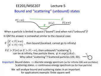
EE201/MSE207 Lecture 8 Measurement and uncertainty principle - PowerPoint PPT Presentation

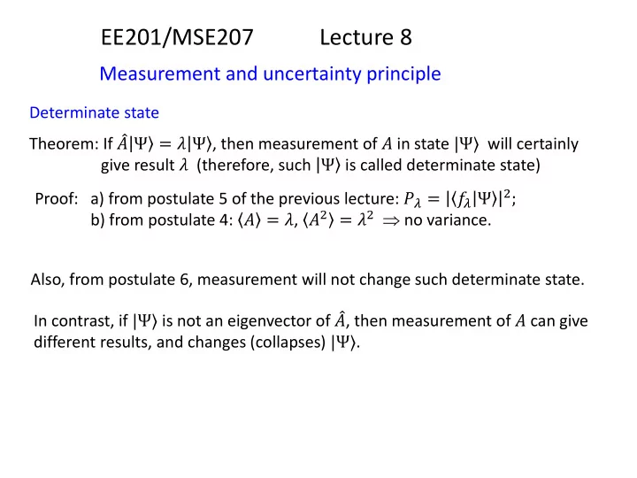
EE201/MSE207 Lecture 8 Measurement and uncertainty principle Determinate state Theorem: If 𝐵 Ψ = 𝜇 Ψ , then measurement of 𝐵 in state |Ψ〉 will certainly give result 𝜇 (therefore, such Ψ is called determinate state) 2 ; Proof: a) from postulate 5 of the previous lecture: 𝑄 𝜇 = 𝑔 𝜇 Ψ b) from postulate 4: 𝐵 = 𝜇 , 𝐵 2 = 𝜇 2  no variance. Also, from postulate 6, measurement will not change such determinate state. In contrast, if |Ψ〉 is not an eigenvector of 𝐵 , then measurement of 𝐵 can give different results, and changes (collapses) |Ψ〉 .

Compatible and incompatible observables Question: When a state can be a determinate state for two operators 𝐵 and 𝐶 ? (why important: consider measurement sequence A , B , A ) Answer: If 𝐶 commute, 𝐵 and 𝐵, 𝐶 = 0 , then this is possible (“compatible”); if 𝐵, 𝐶 ≠ 0 , then this is usually impossible (“incompatible”). More rigorously, two theorems from linear algebra (without proof). Theorem 1 If two Hermitian operators commute, 𝐵, 𝐶 = 0 , then there exists a basis consisting of eigenvectors of both 𝐵 and 𝐶 simultaneously. (These states are determinate states of both 𝐵 and 𝐶 , i.e. 𝜏 𝐵 = 𝜏 𝐶 = 0. ) ( 𝜏 is the standard deviation) Theorem 2 (generalized uncertainty principle) 2 1 2 𝜏 𝐶 2 ≥ 𝐵, 𝜏 𝐶 For Hermitian 𝐵 and 𝐶 , if 𝐵, 𝐶 ≠ 0 , then 𝐵 2𝑗 Example 2 ℏ 𝜏 𝑦 𝜏 𝑞 ≥ ℏ 2 𝜏 𝑞 2 ≥  𝜏 𝑦  𝑦, 𝑞 = 𝑗ℏ 2 2 (Heisenberg uncertainty principle)

Energy-time uncertainty Δ𝐹 Δ𝑢 ≥ ℏ You can often find inequality 2 1) It is formally incorrect, but often gives correct intuition. 2) It is correct in the following sense. Theorem 𝑒〈𝑅〉 𝑒𝑢 ≥ ℏ 𝜏 𝑅 For any observable 𝑅 (which does not 𝜏 𝐹 2 explicitly depend on time) (So, if anything changes significantly during Δ𝑢 , then the energy spread should be large enough, Δ𝐹 Δ𝑢 ≥ ℏ 2 . In stationary state Δ𝐹 = 0 , therefore nothing changes.) 2 1 𝑒〈𝑅〉 = 𝑗 Proof 𝐼, 𝐼, 𝜏 𝐼 𝜏 𝑅 ≥ 𝑅 𝑅 and Straightforward from 2𝑗 𝑒𝑢 ℏ 𝑒𝑢 + Ψ 𝜖 𝑒〈𝑅〉 = 𝑒 𝑅Ψ = 𝑒Ψ 𝑅 𝑒Ψ 𝑅 𝑒𝑢 Ψ 𝑅Ψ + Ψ 𝜖𝑢 Ψ = 𝑒𝑢 𝑒𝑢 𝐼Ψ = 𝑗 = 𝑗 = −𝑗 𝑅 −𝑗 ℏ 𝐼Ψ 𝑅Ψ + Ψ ℏ Ψ 𝐼 𝑅Ψ − Ψ 𝑅 ℏ 〈Ψ| 𝐼, 𝐼Ψ 𝑅 Ψ〉 ℏ 𝑗 ℏ) 〈 𝐼, = ( 𝑅 〉

𝑦 -representation and 𝑞 -representation It is easy to check that both 𝑦 and 𝑞 are Hermitian (as for any observable). We need to prove 𝑔 𝑈𝑕 = 〈 𝑈𝑔|𝑕〉 . 𝑦 this is very simple: 𝑔 ∗ 𝑦 𝑦𝑕 𝑦 𝑒𝑦 = 𝑦 𝑔 𝑦 For ∗ 𝑕 𝑦 𝑒𝑦 . 𝑈 = 𝑞 we need integration by parts: 𝑔 ∗ 𝑦 −𝑗ℏ 𝑒 For 𝑒𝑦 𝑕 𝑦 𝑒𝑦 = 𝑈 = ∗ = 𝑗ℏ 𝑒𝑔 ∗ (𝑦) 𝑕 𝑦 𝑒𝑦 = −𝑗ℏ 𝑒𝑔 𝑦 𝑕 𝑦 𝑒𝑦 . 𝑒𝑦 𝑒𝑦 Find eigenstates of 𝑦 and 𝑞 𝑈𝑔 𝑦 = 𝜇 𝑔(𝑦)  𝑦 𝑔 𝑦 = 𝜇 𝑔(𝑦) 𝑔 𝑦 = 𝐵 𝜀(𝑦 − 𝜇) Eigenstates of 𝑦 : Not normalizable, choose 𝐵 = 1 . 𝑔 𝜇 𝑦 = 𝜀(𝑦 − 𝜇) , then 𝑔 𝜇 𝑔 𝜈 = 𝜀 𝜈 − 𝜇 orthonormal basis Check: 𝜀 𝑦 − 𝜇 𝜀 𝑦 − 𝜈 𝑒𝑦 = 𝜀(𝜈 − 𝜇) (since 𝑦 = 𝜈)

𝑞 : −𝑗ℏ 𝑒 Eigenstates of 𝑕 𝑦 = 𝐶 𝑓 𝑗𝜇  ℏ𝑦 𝑒𝑦 𝑕 𝑦 = 𝜇 𝑕(𝑦) 2𝜌ℏ 𝑓 𝑗 𝜇 1 ℏ 𝑦 , then 𝑕 𝜇 𝑕 𝜈 = 𝜀 𝜈 − 𝜇 𝑕 𝜇 𝑦 = orthonormal basis 2𝜌ℏ 𝑓 −𝑗 𝜇 ℏ 𝑦 𝑓 𝑗 𝜈 2𝜌ℏ 𝑓 𝑗 𝜈−𝜇 ℏ 𝑦 𝑒𝑦 = ℏ 𝑦 𝑒𝑦 = 𝜀(𝜈 − 𝜇) Check: 1 1 ∞ 𝑓 𝑗𝑙𝑦 𝑒𝑦 = 2𝜌 𝜀 𝑙 and 𝜀 𝑏𝑦 = 𝜀(𝑦) since −∞ |𝑏| ∞ 𝑓 𝑗𝑙𝑦 𝑒𝑦 = 2𝜌 𝜀 𝑙 Digression: proof of the formula −∞ 2𝜌 𝑓 −𝑗𝑙𝑦 𝑔 𝑦 𝑒𝑦 1 1 2𝜌 𝑓 𝑗𝑙𝑦 𝐺 𝑙 𝑒𝑙 , 𝐺 𝑙 = Fourier transform 𝑔 𝑦 = Therefore 1 1 1 𝑓 𝑗𝑙 ′ 𝑦 𝐺 𝑙′ 𝑒𝑙 ′ = 2𝜌 𝑓 𝑗 𝑙 ′ −𝑙 𝑦 𝑒𝑦 𝐺 𝑙 ′ 𝑒𝑙 𝑒𝑦 𝑓 −𝑗𝑙𝑦 𝐺 𝑙 = 2𝜌 2𝜌 𝜀(𝑙 − 𝑙 ′ )

Similarity of 𝑦 -representation and 𝑞 -representation 1 𝑓 𝑗𝜇 ℏ𝑦 𝑔 𝜇 𝑦 = 𝜀(𝑦 − 𝜇) 𝑦 -eigenstates 𝑞 -eigenstates 𝑕 𝜇 𝑦 = 2𝜌ℏ ( x -basis) ( p -basis) We can say that Ψ 𝑦 are actually components of vector |Ψ〉 in x -basis: ∞ Ψ 𝑦 ′ 𝜀 𝑦 − 𝑦 ′ 𝑒𝑦 ′ Ψ 𝑦 = −∞ basis vectors components Similarly, we can write it in p -basis: ∞ 1 𝑓 𝑗𝑞 ∞ ℏ𝑦 𝑒𝑞 1 𝑓 −𝑗𝑞 ℏ 𝑦 Ψ 𝑦 𝑒𝑦 Ψ 𝑦 = Φ 𝑞 Φ 𝑞 = 2𝜌ℏ 2𝜌ℏ −∞ −∞ basis vectors components We can regard Φ 𝑞 as a wavefunction in p -space Actually, more often people use Φ 𝑙 in 𝑙 -space, where 𝑙 = 𝑞/ℏ , then eigenstates (basis vectors) are 1 2𝜌 𝑓 𝑗𝑙𝑦 .

Operators 𝑦 and 𝑞 in p -space 𝑞Φ 𝑞 = 𝑞 Φ(𝑞) −𝑗ℏ 𝜖Ψ(𝑦) = −𝑗ℏ 𝜖 1 𝑓 𝑗𝑞 ℏ 𝑦 𝑒𝑞 = 𝜖𝑦 Φ 𝑞 Expected by analogy. Formal proof: 𝜖𝑦 2𝜌ℏ 1 𝑗𝑞 1 ℏ 𝑓 𝑗𝑞 𝑓 𝑗𝑞 ℏ𝑦 𝑒𝑞 = 𝑞 Φ 𝑞 ℏ𝑦 𝑒𝑞 = −𝑗ℏ Φ 𝑞 2𝜌ℏ 2𝜌ℏ 𝑦Φ 𝑞 = 𝑗ℏ 𝜖 1 𝜖𝑞 Φ(𝑞) 𝑦 𝑓 𝑗𝑞 ℏ𝑦 𝑒𝑞 = Proof: 𝑦Ψ(𝑦) = Φ 𝑞 2𝜌ℏ −𝑗ℏ 𝜖 𝜖𝑞 𝑓 𝑗𝑞 ℏ𝑦 = by parts = 𝑗ℏ 𝑒Φ(𝑞) 1 𝑓 𝑗𝑞 ℏ𝑦 𝑒𝑞 𝑒𝑞 2𝜌ℏ 𝑞 = 𝑦, −𝑗ℏ 𝜖 𝑦, 𝜖𝑦 = 𝑗ℏ Commutator does not change 𝑞 = 𝑗ℏ 𝜖 𝑦, 𝜖𝑞 , 𝑞 = 𝑗ℏ

2 𝑒𝑦 and Φ 𝑞 2 𝑒𝑞 Probabilities Ψ 𝑦 Φ 𝑞 is as good a wavefunction as Ψ 𝑦 For x -measurement, probability to find particle near 𝑦 0 is 𝒬 𝑦 0 𝑒𝑦 (postulate 5, rem. a), with 2 = 𝜀 𝑦 − 𝑦 0 Ψ 𝑦 𝑒𝑦 2 = Ψ 𝑦 0 2 𝒬 𝑦 0 = 𝑔 𝑦 0 Ψ Similarly, for p -measurement, probability to find momentum near 𝑞 0 is 𝒬 𝑞 0 𝑒𝑞 , with 2 2 = 2𝜌ℏ e −𝑗 𝑞0 ℏ 𝑦 Ψ 𝑦 𝑒𝑦 1 2 𝒬 𝑞 0 = 𝑕 𝑞 0 Ψ = Φ 𝑞 0

Minimum-uncertainty states From Heisenberg uncertainty relation, we know that 𝜏 𝑦 𝜏 𝑞 ≥ ℏ 2 Which states satisfy the lower bound, 𝜏 𝑦 𝜏 𝑞 = ℏ 2 ? Answer: 1/4 𝑏 Ψ 𝑦 = 𝐵 𝑓 −𝑏 𝑦−𝑦 0 2 /2ℏ 𝑓 𝑗𝑞 0 𝑦/ℏ 𝐵 = 𝜌ℏ (in optics they are called “squeezed states”) ℏ 𝑏ℏ 𝜏 𝑦 = 2𝑏 , It has 𝑦 = 𝑦 0 , 𝑞 = 𝑞 0 , 𝜏 𝑞 = 2 , In p -representation very similar form: 1 ℏ𝑦 Ψ 𝑦 𝑒𝑦 = 𝑓 𝑗𝑞 0 𝑦 0 /ℏ 𝐵 𝑓 −𝑗 𝑞 𝑏 𝑓 − 𝑞−𝑞 0 2 /(2ℏ𝑏) 𝑓 −𝑗𝑦 0 𝑞/ℏ Φ 𝑞 = 2𝜌ℏ