SLIDE 1
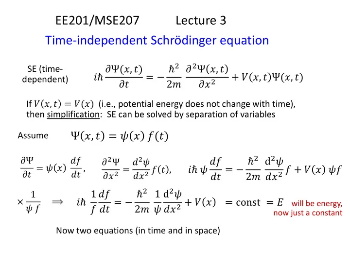
will be energy, now just a constant
EE201/MSE207 Lecture 3
SE (time- dependent)
𝑗ℏ 𝜖Ψ(𝑦, 𝑢) 𝜖𝑢 = − ℏ2 2𝑛 𝜖2Ψ 𝑦, 𝑢 𝜖𝑦2 + 𝑊 𝑦, 𝑢 Ψ(𝑦, 𝑢)
Time-independent Schrödinger equation
If 𝑊 𝑦, 𝑢 = 𝑊(𝑦) (i.e., potential energy does not change with time), then simplification: SE can be solved by separation of variables Assume
Ψ 𝑦, 𝑢 = 𝜔 𝑦 𝑔(𝑢)
𝜖Ψ 𝜖𝑢 = 𝜔 𝑦 𝑒𝑔 𝑒𝑢 , 𝜖2Ψ 𝜖𝑦2 = 𝑒2𝜔 𝑒𝑦2 𝑔 𝑢 ,
𝑗ℏ 𝜔 𝑒𝑔 𝑒𝑢 = − ℏ2 2𝑛 d2𝜔 𝑒𝑦2 𝑔 + 𝑊 𝑦 𝜔𝑔
× 1 𝜔 𝑔 ⟹
𝑗ℏ 1 𝑔 𝑒𝑔 𝑒𝑢 = − ℏ2 2𝑛 1 𝜔 d2𝜔 𝑒𝑦2 + 𝑊 𝑦 = const
Now two equations (in time and in space)
= 𝐹
SLIDE 2
𝑒𝑔 𝑒𝑢 = −𝑗 𝐹 ℏ 𝑔
⟹
𝑗ℏ 1 𝑔 𝑒𝑔 𝑒𝑢 = − ℏ2 2𝑛 1 𝜔 d2𝜔 𝑒𝑦2 + 𝑊 𝑦 = 𝐹
First equation:
𝑔 𝑢 = 𝐷 𝑓
−𝑗𝐹 ℏ 𝑢
Can choose 𝐷 = 1 𝐹 must be real (for normalization)
Ψ 𝑦, 𝑢 = 𝜔 𝑦 𝑔(𝑢) 𝑔 𝑢 = exp −𝑗 𝐹 ℏ 𝑢
Second equation:
− ℏ2 2𝑛 d2𝜔 𝑦 𝑒𝑦2 + 𝑊 𝑦 𝜔 𝑦 = 𝐹 𝜔 𝑦
Time-independent Schrödinger equation (TISE)
𝐼𝜔 = 𝐹 𝜔
(this hints that E is energy)
Ψ 𝑦, 𝑢 = 𝜔 𝑦 exp −𝑗 𝐹 ℏ 𝑢
Normalization
−∞ ∞
Ψ 2𝑒𝑦 = 1,
while exp −𝑗 𝐹 ℏ 𝑢 = 1 therefore
−∞ ∞
𝜔(𝑦) 2𝑒𝑦 = 1 𝜔 normalized in the same way as Ψ
SLIDE 3
𝑅 =
−∞ ∞ 𝜔 𝑦 𝑓 −𝑗𝐹𝑢 ℏ ∗𝑅 𝑦, −𝑗ℏ 𝜖 𝜖𝑦 [𝜔 𝑦 𝑓 −𝑗𝐹𝑢 ℏ] 𝑒𝑦
For any observable 𝑅(𝑦, 𝑞) , the average 𝑅(𝑦, −𝑗ℏ 𝜖 𝜖𝑦) does not depend on time ⇒ stationary state time-dependence cancels
Ψ 𝑦, 𝑢 = 𝜔 𝑦 exp −𝑗 𝐹 ℏ 𝑢
Stationary state
Let us show that E is energy
𝐼𝜔 = 𝐹𝜔
Average energy:
𝐼 =
−∞ ∞ 𝜔∗
𝐼𝜔 𝑒𝑦 =
−∞ ∞ 𝜔∗𝐹𝜔 𝑒𝑦 =
= 𝐹
−∞ ∞ 𝜔 2 𝑒𝑦 = 𝐹
Similarly
𝐼2 =
−∞ ∞ 𝜔∗
𝐼 𝐼𝜔 𝑒𝑦 =
−∞ ∞ 𝜔∗𝐹𝐹𝜔 𝑒𝑦 = 𝐹2
No variance ⟹ energy is E (definite energy, “well-defined” energy, rare case in QM)
(H is operator of total energy)
SLIDE 4
TISE solutions (infinitely many): SE is linear ⟹ any linear combination of solutions is a solution
− ℏ2 2𝑛 d2𝜔𝑜 𝑒𝑦2 + 𝑊(𝑦) 𝜔𝑜 = 𝐹𝑜 𝜔𝑜 Ψ 𝑦, 𝑢 =
𝑜=1 ∞
𝑑𝑜 𝜔𝑜 𝑦 exp −𝑗 𝐹𝑜 ℏ 𝑢 𝑜 = 1, 2, 3, …
General solution of SE (for time-independent 𝑊(𝑦))
Any complex coefficients 𝑑𝑜 ; however, Ψ should be normalized. As we will see, with normalized 𝜔𝑜, this requires normalization for 𝑑𝑜 as
𝑜=1 ∞
𝑑𝑜 2 = 1
SLIDE 5 Theorem
Stationary states 𝜔𝑜(𝑦) and 𝜔𝑛 𝑦 with different energies,
𝐹𝑜 ≠ 𝐹𝑛 , are orthogonal:
−∞ ∞ 𝜔𝑛 ∗ 𝑦 𝜔𝑜 𝑦 𝑒𝑦 = 0.
Orthogonality of stationary states
Remarks: - orthonormal (since normalized)
- we treat functions as vectors, inner product (generalized dot-product)
𝑔 ≡
−∞ ∞ 𝑔∗ 𝑦 𝑦 𝑒𝑦, orthogonal: 𝑔 = 0
Proof Start with − ℏ2
2𝑛 d2𝜔𝑜 𝑒𝑦2 + 𝑊 𝜔𝑜 = 𝐹𝑜 𝜔𝑜
× 𝜔𝑛
∗ , integrate: − ℏ2
2𝑛 𝜔𝑛 ∗ d2𝜔𝑜 𝑒𝑦2 𝑒𝑦 + 𝜔𝑛 ∗ 𝑊𝜔𝑜𝑒𝑦 = 𝐹𝑜 𝜔𝑛 ∗ 𝜔𝑜𝑒𝑦
exchange 𝑜 ↔ 𝑛,
conjugate:
− ℏ2
2𝑛 𝜔𝑜 d2𝜔𝑛
∗
𝑒𝑦2 𝑒𝑦 + 𝜔𝑜𝑊𝜔𝑛 ∗ 𝑒𝑦 = 𝐹𝑛 𝜔𝑜𝜔𝑛 ∗ 𝑒𝑦
equal (by parts) equal
⇒ also equal
(𝐹𝑜−𝐹𝑛) 𝜔𝑛
∗ 𝜔𝑜𝑒𝑦 = 0
If 𝐹𝑜 ≠ 𝐹𝑛, then 𝜔𝑛
∗ 𝜔𝑜𝑒𝑦 = 0
Q.E.D. If energies are the same, usually also choose orthogonal functions 𝜔𝑜(𝑦)
SLIDE 6 Normalization for coefficients 𝑑𝑜
Use orthogonality of 𝜔𝑜
Ψ 𝑦, 𝑢 =
𝑜=1 ∞
𝑑𝑜 𝜔𝑜 𝑦 exp −𝑗 𝐹𝑜 ℏ 𝑢 1 =
−∞ ∞
Ψ(𝑦, 𝑢) 2𝑒𝑦 =
𝑜,𝑛
𝑑𝑛
∗ 𝑑𝑜 exp −𝑗 𝐹𝑜 − 𝐹𝑛
ℏ 𝑢
−∞ ∞
𝜔𝑛
∗ 𝑦 𝜔𝑜 𝑦 𝑒𝑦
=
𝑜
𝑑𝑜 2 × 1 ×
−∞ ∞
𝜔𝑜 𝑦
2𝑒𝑦 = 𝑜
𝑑𝑜 2
This is how we obtain normalization for 𝑑𝑜:
𝑜=1 ∞
𝑑𝑜 2 = 1
SLIDE 7
General solution for evolution of Ψ(𝑦, 𝑢)
Ψ 𝑦, 𝑢 =
𝑜=1 ∞
𝑑𝑜 𝜔𝑜 𝑦 exp −𝑗 𝐹𝑜 ℏ 𝑢 𝜀𝑜𝑛
Suppose we know wave function at 𝑢 = 0: Ψ(𝑦, 0) Then we can find coefficients 𝑑𝑜 in Ψ 𝑦, 0 = 𝑜 𝑑𝑜𝜔𝑜 𝑦 Again use orthogonality: multiply by 𝜔𝑛
∗ (𝑦) and integrate
𝜔𝑛
∗ 𝑦 Ψ 𝑦, 0 𝑒𝑦 = 𝑜 𝑑𝑜 𝜔𝑛 ∗ 𝑦 𝜔𝑜 𝑦 𝑒𝑦 = 𝑑𝑛
Therefore
𝑑𝑜 =
−∞ ∞ 𝜔𝑜 ∗ 𝑦 Ψ 𝑦, 0 𝑒𝑦
Then we can find Ψ(𝑦, 𝑢) at any time 𝑢 :
SLIDE 8 Example: Infinite square well
𝑙 = 2𝑛𝐹 ℏ
(one of the most important systems in this course) Boundary conditions: x
a 𝑊 𝑦 = 0, 0 ≤ 𝑦 ≤ 𝑏 ∞,
(similar to quantum well in semiconductors, except different effective mass and finite depth) Solve TISE inside
− ℏ2 2𝑛 d2𝜔 𝑦 𝑒𝑦2 = 𝐹 𝜔 𝑦 ⇒ 𝜔 𝑦 = 𝐵 sin 𝑙𝑦 + 𝐶 cos(𝑙𝑦) 𝜔 0 = 0 𝜔 𝑏 = 0
(because 𝜔 𝑦 = 0 outside and 𝜔(𝑦) is always continuous)
𝜔 𝑦 = 𝐵 sin 𝑙𝑜𝑦
therefore
𝑙𝑜 = 𝜌𝑜 𝑏 , 𝑜 = 1, 2, 3, … 𝐹𝑜 = ℏ2𝑙𝑜
2
2𝑛 = 𝑜2𝜌2ℏ2 2𝑛𝑏2 𝑊(𝑦)
SLIDE 9 Infinite square well
x
a 𝜔𝑜 𝑦 = 𝐵 sin 𝑙𝑜𝑦 , 𝑙𝑜 = 𝑜𝜌 𝑏 𝐹𝑜 = ℏ2𝑙𝑜
2
2𝑛 = 𝑜2𝜌2ℏ2 2𝑛𝑏2 𝑜 = 1, 2, 3, …
Normalization
1 =
𝑏 𝜔 𝑦 2𝑒𝑦 = 𝐵 2 1 2 𝑏 ⇒ 𝐵 =
2 𝑏
𝜔𝑜 𝑦 = 2 𝑏 sin 𝑜𝜌 𝑏 𝑦
(because sin2(𝑦) = 1/2)
n=1 – lowest energy,
“ground state”
n2 – “excited states”
Similar to atom states Even lowest state has positive energy (understanding
from uncertainty principle)
𝑊(𝑦)
1
n=1 n=2 n=3 a 𝜔𝑜(𝑦)
SLIDE 10 Infinite square well: Summary
x
a
𝐹𝑜 = 𝑜2𝜌2ℏ2 2𝑛𝑏2
𝑜 = 1, 2, 3, …
𝜔𝑜 𝑦 = 2 𝑏 sin 𝑜𝜌 𝑏 𝑦
n=1 – lowest energy,
“ground state”
n2 – “excited states” 𝑊(𝑦) 𝑙𝑜 = 𝑜𝜌 𝑏
4 9
n=1 n=2 n=3 𝐹1 𝐹2 𝐹3
1
n=1 n=2 n=3 a 𝜔𝑜(𝑦)
SLIDE 11 Infinite square well: properties of stationary states
x
a 𝑜 = 1, 2, 3, … 𝜔𝑜 𝑦 = 2 𝑏 sin 𝑜𝜌 𝑏 𝑦 𝑊(𝑦) orthogonal to each other,
𝑏 𝜔𝑛 ∗ 𝑦 𝜔𝑜(𝑦) 𝑒𝑦 = 𝜀𝑛𝑜
complete set, any 𝑔 𝑦 can be represented as 𝑔 𝑦 = 𝑜=1
∞
𝑑𝑜 𝜔𝑜 𝑦
if 𝑔 0 = 𝑔 𝑏 = 0 How to find 𝑑𝑜? Already know the trick:
𝜔𝑛
∗ 𝑦 𝑔(𝑦) 𝑒𝑦 = 𝑜 𝑑𝑜 𝜔𝑛 ∗ 𝑦 𝜔𝑜 𝑦 𝑒𝑦 = 𝑑𝑛
Therefore
𝑑𝑜 =
𝑏
𝜔𝑜
∗ 𝑦 𝑔(𝑦) 𝑒𝑦
(i.e., orthonormal basis)
1
n=1 n=2 n=3 a 𝜔𝑜(𝑦)
SLIDE 12 General solution
x
a 𝑊(𝑦)
4 9
n=1 n=2 n=3 𝐹1 𝐹2 𝐹3 Ψ 𝑦, 𝑢 =
𝑜=1 ∞
𝑑𝑜 2 𝑏 sin 𝑜𝜌 𝑏 𝑦 exp −𝑗 𝑜2𝜌2ℏ 2𝑛𝑏2 𝑢 𝑜=1
∞
𝑑𝑜 2 = 1
If only one coefficient 𝑑𝑜 is non-zero, then stationary state If more than one level occupied (“superposition”), then non-stationary, state evolves in time (interference) Classical motion can be represented as combination
- f many high-numbered states (transition to classical
picture when energies are ≫ 𝐹1,2,3) Is a general (superposition) state localized in space? – No Is it localized in energy? – Also no! However, if we measure energy, then we will get some result: some 𝐹𝑜 (nothing in between!) If measure again – will get the same result (collapse)