6.1 Inner Product, Length & Orthogonality Not all linear - - PDF document

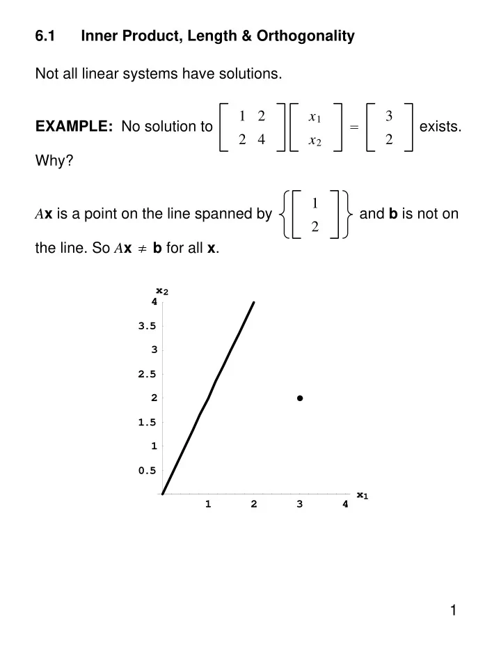
6.1 Inner Product, Length & Orthogonality Not all linear systems have solutions. EXAMPLE: No solution to 1 2 2 4 x1 x2 = 3 2 exists. Why? Ax is a point on the line spanned by 1 2 and b is not on the line. So Ax ≠ b for all x.

1 2 3 4 x1 0.5 1 1.5 2 2.5 3 3.5 4 x2

1

Instead find  x so that A x lies ”closest” to b.

1 2 3 4 x1 0.5 1 1.5 2 2.5 3 3.5 4 x2

Using information we will learn in this chapter, we will find that  x= 1.4 , so that A x =

• 1. 4
• 2. 8

. Segment joining A x and b is perpendicular (or orthogonal) to the set of solutions to Ax = b. Need to develop fundamental ideas of length, orthogonality and

• rthogonal projections.

2

The Inner Product Inner product or dot product of u = u1 u2 ⋮ un and v = v1 v2 ⋮ vn : u ⋅ v = uTv = u1 u2 ⋯ un v1 v2 ⋮ vn = u1v1 + u2v2 + ⋯ + unvn Note that v ⋅ u =v1u1 + v2u2 + ⋯ + vnun = u1v1 + u2v2 + ⋯ + unvn = u ⋅ v 3

THEOREM 1 Let u,v and w be vectors in Rn, and let c be any scalar. Then

• a. u ⋅ v = v ⋅ u
• b. u + v ⋅ w = u ⋅ w + v ⋅ w
• c. cu ⋅ v =cu ⋅ v= u ⋅ cv
• d. u ⋅ u ≥ 0, and u ⋅ u = 0 if and only if u = 0.

Combining parts b and c, one can show c1u1 + ⋯ + cpup ⋅ w =c1u1 ⋅ w + ⋯ + cpup ⋅ w 4

Length of a Vector For v = v1 v2 ⋮ vn , the length or norm of v is the nonnegative scalar ‖v‖ defined by ‖v‖ = v ⋅ v = v1

2 + v2 2 + ⋯ + vn 2

and ‖v‖2 = v ⋅ v. For example, if v = a b , then ‖v‖ = a2 + b2 (distance between 0 and v) Picture: For any scalar c, ‖cv‖ = |c|‖v‖ 5

Distance in Rn The distance between u and v in Rn: distu,v = ‖u − v‖. This agrees with the usual formulas for R2 and R3. Let u =u1,u2 and v =v1,v2. Then u − v =u1 − v1,u2 − v2 and distu,v = ‖u − v‖ = ‖u1 − v1,u2 − v2‖ = u1 − v12 + u2 − v22 6

Orthogonal Vectors distu,v2 = ‖u − v‖2 = u − v ⋅ u − v = u ⋅ u − v + −v ⋅ u − v = = u ⋅ u − u ⋅ v + −v ⋅ u + v ⋅ v =‖u‖2 + ‖v‖2 − 2u ⋅ v ⇒ distu,v2 = ‖u‖2 + ‖v‖2 − 2u ⋅ v Similarly, distu,−v2 = ‖u‖2 + ‖v‖2 + 2u ⋅ v 7

Since distu,−v2 = distu,v2, u ⋅ v = ___. Two vectors u and v are said to be orthogonal (to each other) if u ⋅ v = 0. Also note that if u and v are orthogonal, then ‖u + v‖ = ‖u‖2 + ‖v‖2. THEOREM 2 THE PYTHAGOREAN THEOREM Two vectors u and v are orthogonal if and only if ‖u + v‖ = ‖u‖2 + ‖v‖2. 8

Orthogonal Complements If a vector z is orthogonal to every vector in a subspace W of Rn, then z is said to be orthogonal to W. The set of vectors z that are orthogonal to W is called the orthogonal complement of W and is denoted by W⊥ (read as “W perp”). 9

Row, Null and Columns Spaces THEOREM 3 Let A be an m × n matrix. Then the orthogonal complement

• f the row space of A is the nullspace of A, and the
• rthogonal complement of the column space of A is the

nullspace of AT: Row A

⊥ =Nul A,

Col A

⊥ =Nul AT.

Why? (See complete proof in the text) Consider Ax = 0: ∗ ∗ ⋯ ∗ ∗ ∗ ⋯ ∗ ⋮ ⋮ ⋱ ⋮ ∗ ∗ ⋯ ∗ ⋆ ⋆ ⋮ ⋆ = ⋮ Note that Ax = r1 ⋅ x r2 ⋅ x ⋮ rm ⋅ x = ⋮ and so x is orthogonal to the row A since x is orthogonal to r1.…,rm. 10

EXAMPLE: Let A = 1 0 −1 2 0 2 . Basis for Nul A = 1 , 1 1 and therefore Nul A is a plane in R3. Basis for Row A = 1 −1 and therefore Row A is a line in R3. Basis for Col A = 1 2 and therefore Col A is a line in R2. Basis for Nul AT = −2 1 and therefore Nul AT is a line in R2. 11

Subspaces Nul A and Row A

−4 −2

2 4 x1

−4 −2

2 4 x2

Subspaces Nul AT and Col A 12