Perturbation theory (Ch. 6) (time-independent, nondegenerate, Sec. - PowerPoint PPT Presentation

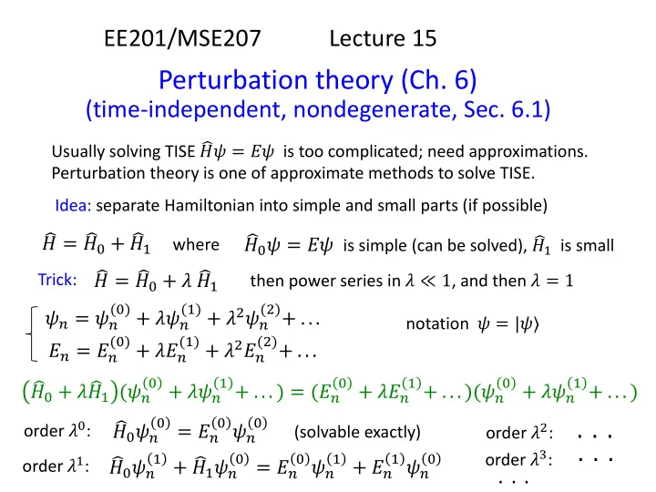
EE201/MSE207 Lecture 15 Perturbation theory (Ch. 6) (time-independent, nondegenerate, Sec. 6.1) Usually solving TISE 𝐼𝜔 = 𝐹𝜔 is too complicated; need approximations. Perturbation theory is one of approximate methods to solve TISE. Idea: separate Hamiltonian into simple and small parts (if possible) 𝐼 = 𝐼 0 + 𝐼 0 𝜔 = 𝐹𝜔 is simple (can be solved), 𝐼 1 𝐼 1 is small where 𝐼 = 𝐼 0 + 𝜇 𝐼 1 then power series in 𝜇 ≪ 1 , and then 𝜇 = 1 Trick: (0) + 𝜇𝜔 𝑜 (1) + 𝜇 2 𝜔 𝑜 (2) + . . . 𝜔 𝑜 = 𝜔 𝑜 notation 𝜔 = |𝜔〉 (0) + 𝜇𝐹 𝑜 (1) + 𝜇 2 𝐹 𝑜 (2) + . . . 𝐹 𝑜 = 𝐹 𝑜 0 + 𝜇𝜔 𝑜 1 + . . . ) = (𝐹 𝑜 0 + 𝜇𝐹 𝑜 1 + . . . )(𝜔 𝑜 0 + 𝜇𝜔 𝑜 1 + . . . ) 𝐼 0 + 𝜇 𝐼 1 (𝜔 𝑜 0 = 𝐹 𝑜 0 𝜔 𝑜 0 . . . order 𝜇 0 : 𝐼 0 𝜔 𝑜 order 𝜇 2 : (solvable exactly) . . . 1 + 0 = 𝐹 𝑜 0 𝜔 𝑜 1 + 𝐹 𝑜 1 𝜔 𝑜 order 𝜇 3 : 0 order 𝜇 1 : 𝐼 0 𝜔 𝑜 𝐼 1 𝜔 𝑜 . . .

First-order perturbation theory ( 𝜇 1 ) 1 + 0 = 𝐹 𝑜 0 𝜔 𝑜 1 + 𝐹 𝑜 1 𝜔 𝑜 0 𝐼 0 𝜔 𝑜 𝐼 1 𝜔 𝑜 ∗ ∞ 𝑒𝑦 , or (the same) 〈𝜔 𝑜 0 𝑦 0 |. . . Multiply by 𝜔 𝑜 and integrate, −∞ 1 〉 + 〈𝜔 𝑜 0 | 0 〉 = 𝐹 𝑜 0 〈𝜔 𝑜 0 |𝜔 𝑜 1 〉 + 𝐹 𝑜 (0) | 1 〈𝜔 𝑜 𝐼 0 |𝜔 𝑜 𝐼 1 |𝜔 𝑜 equal notation 𝜔 1 𝐼 𝜔 2 = 〈𝜔 1 | 𝐼 𝜔 2 〉 1 = 〈𝜔 𝑜 0 | 0 〉 𝐹 𝑜 𝐼 1 |𝜔 𝑜 First-order correction to energy is just the average (expectation) value of 𝐼 1 in the unperturbed state (very natural)

First-order perturbation theory (cont.) 1 + 0 = 𝐹 𝑜 0 𝜔 𝑜 1 + 𝐹 𝑜 1 𝜔 𝑜 0 𝐼 0 𝜔 𝑜 𝐼 1 𝜔 𝑜 (1) to wavefunction Now find correction 𝜔 𝑜 0 ) 𝜔 𝑜 1 = −( (1) ) 𝜔 𝑜 0 ( 𝐼 0 − 𝐹 𝑜 𝐼 1 −𝐹 𝑜 Rewrite (1) = 𝑛≠𝑜 𝑑 𝑛 (𝑜) 𝜔 𝑛 (𝑜) = 0 (0) 𝜔 𝑜 𝑑 𝑜 Expand in zero-order eigenstates from normalization (0) − 𝐹 𝑜 (𝑜) 𝜔 𝑛 0 ) 𝑑 𝑛 0 = −( (1) ) 𝜔 𝑜 0 𝑛≠𝑜 (𝐹 𝑛 𝐼 1 −𝐹 𝑜 0 − 𝐹 𝑜 0 ) 𝑑 𝑚 𝑜 = − 𝜔 𝑚 1 𝜀 𝑚𝑜 0 0 (0) | : (𝐹 𝑚 𝐼 1 𝜔 𝑜 + 𝐹 𝑜 Multiply by 〈𝜔 𝑚 (1) (another way of derivation) For 𝑜 = 𝑚 we obtain the previous formula for 𝐹 𝑜 0 0 𝑜 = 𝜔 𝑚 𝐼 1 𝜔 𝑜 For 𝑜 ≠ 𝑚 : 𝑑 𝑚 0 − 𝐹 𝑚 0 𝐹 𝑜 0 0 𝜔 𝑛 𝐼 1 𝜔 𝑜 (1) = (0) 𝜔 𝑜 𝜔 𝑛 0 − 𝐹 𝑛 0 Rename 𝑚 → 𝑛 𝐹 𝑜 𝑛≠𝑜

First-order perturbation theory: summary 𝐼 = 𝐼 0 + 𝐼 1 1 = 〈𝜔 𝑜 0 | 0 〉 𝐹 𝑜 𝐼 1 |𝜔 𝑜 0 = 𝐹 𝑜 0 𝜔 𝑜 0 𝐼 0 𝜔 𝑜 (0) + 𝜔 𝑜 (1) + … 0 0 𝜔 𝑛 𝐼 1 𝜔 𝑜 𝜔 𝑜 = 𝜔 𝑜 (1) = (0) 𝜔 𝑜 𝜔 𝑛 0 − 𝐹 𝑛 0 (0) + 𝐹 𝑜 (1) + … 𝐹 𝑜 𝐹 𝑜 = 𝐹 𝑜 𝑛≠𝑜 (0) = 𝐹 𝑜 (0) (i.e. when degeneracy). Then Remark. Correction to 𝜔 𝑜 is not good if 𝐹 𝑛 the formalism is a little different. Usually degeneracy is lifted (disappears) due to perturbation. For example, in hydrogen atom there is fine structure (due to relativistic correction and spin-orbit) and hyperfine structure (due to magnetic interaction of electron and proton). Second-order perturbation: similar but lengthier 2 Result for second-order correction 0 0 𝜔 𝑛 𝐼 1 𝜔 𝑜 (2) = to energy of n th level: 𝐹 𝑜 0 − 𝐹 𝑛 0 𝐹 𝑜 𝑛≠𝑜

WKB approximation (Ch. 8) (Wentzel, Kramers, Brillouin, 1926) − ℏ 2 𝑒 2 𝜔 𝑦 𝐹 can be discrete + 𝑊 𝑦 𝜔 𝑦 = 𝐹 𝜔(𝑦) 𝑒𝑦 2 2𝑛 or continuous If 𝑊 𝑦 = const , then easy to solve If 𝑊 𝑦 varies slowly, then modify solution for 𝑊 𝑦 = const . Idea: Two cases: 𝐹 > 𝑊(𝑦) (classical region) 𝐹 < 𝑊(𝑦) (tunneling)

WKB approximation, classical region, 𝐹 > 𝑊(𝑦) 2𝑛(𝐹 − 𝑊) If 𝑊 𝑦 = const = 𝑊 , then 𝜔 𝑦 = 𝐵 𝑓 ±𝑗𝑙𝑦 , 𝑙 = ℏ 𝑦 𝑙 𝑦 ′ 𝑒𝑦 ′ Then for 𝑊(𝑦) we expect 𝜔 𝑦 ≈ 𝐵 𝑦 exp ±𝑗 2𝑛 𝜔 𝑒𝜔 ∗ 𝐾 = 𝑗ℏ 𝑒𝑦 − 𝜔 ∗ 𝑒𝜔 From conservation of the probability current 𝑒𝑦 1 𝐵 𝑦 ∝ we obtain Therefore 𝑙(𝑦) 𝑦 𝜔 𝑦 ≈ const 𝑙 𝑦 ′ 𝑒𝑦 ′ 2𝑛[𝐹 − 𝑊 𝑦 ] exp ±𝑗 𝑙(𝑦) = 𝑙 𝑦 ℏ 𝑗 slightly different in the textbook, ± ℏ 𝑞 𝑦 𝑒𝑦 𝑤 𝑦 , so 𝜔 2 ∝ Remark 1. 1 𝑙(𝑦) ∝ 1 1 𝑤(𝑦) , as it should be. Remark 2. If 𝑛(𝑦) (as in SiGe technology), then 𝐵(𝑦) ∝ 𝑛(𝑦) 𝑙(𝑦) . Remark 3. WKB approximation works well only for slowly changing 𝑊(𝑦) .

WKB approximation, tunneling, 𝐹 < 𝑊(𝑦) 2𝑛(𝑊 − 𝐹) If 𝑊 𝑦 = const = 𝑊 , then 𝜔 𝑦 = 𝐵 𝑓 ±𝜇𝑦 , 𝜇 = ℏ Similarly 𝑦 𝜔 𝑦 ≈ const 𝜇 𝑦 ′ 𝑒𝑦 ′ 2𝑛[𝑊 𝑦 − 𝐹] exp ± 𝜇(𝑦) = 𝜇 𝑦 ℏ WKB approximation is often used to estimate probability of tunneling (coefficient of transmission) through a strong (almost “opaque”) tunnel barrier 𝑊(𝑦) Tunneling probability 𝜔 𝑗𝑜 𝜔 𝑝𝑣𝑢 𝜔 out 2 𝜔 in 2 𝑈 ≃ 𝐹 𝑈 ⋘ 1 𝑏 𝜇 𝑦 𝑒𝑦) 0 𝑈 ≃ exp(−2 𝑏 0 (very crudely; we neglect all pre-exponential factors, which usually are within one order of magnitude, while exponential factor can typically be 10 −3 − 10 −10 )

WKB, connection between the two regions assume smooth 𝑊(𝑦) 𝐹 (different result for an abrupt potential) 𝑊(𝑦) 𝑦 0 (classical turning point) WKB approximation does not work well in the vicinity of 𝑦 0 , we need a better approximation near 𝑦 0 (linear potential, Airy functions). Result: 𝑦 𝐷 𝜇 𝑦 ′ 𝑒𝑦′ , exp − 𝑦 > 𝑦 0 𝜇(𝑦) 𝑦 0 𝜔 𝑦 ≈ 𝑦 0 2 𝐷 sin 𝜌 𝑙 𝑦 ′ 𝑒𝑦′ , 4 + 𝑦 < 𝑦 0 𝑙(𝑦) 𝑦

Variational principle (Ch. 7) Only Sec. 7.1 Theorem: For an arbitrary |𝜔〉 , the ground state energy 𝐹 𝑕 satisfies inequality 𝐹 𝑕 ≤ 𝜔 𝐼 𝜔 = 〈 𝐼〉 Proof is simple. Let us expand 𝜔 = 𝑜 𝑑 𝑜 |𝜔 𝑜 〉 . Then since 𝐹 𝑜 ≥ 𝐹 𝑕 , we get 𝐼 = 𝑜 𝑑 𝑜 2 𝐹 𝑜 ≥ 𝐹 𝑕 𝑜 𝑑 𝑜 2 = 𝐹 𝑕 This theorem can be useful to estimate 𝐹 𝑕 (or at least to find an upper bound) Idea: Use trial wavefunctions |𝜔〉 with many adjustable parameters and minimize 〈 𝐼〉 . Hopefully min 〈 𝐼〉 is close to 𝐹 𝑕 . Extensions of this method can also be used to find |𝜔 𝑕 〉 , first-excited state energy and wavefunction (using subspace orthogonal to |𝜔 𝑕 〉 ), second-excited state, etc.