EE201/MSE207 Lecture 9 Quantum mechanics in three dimensions - PowerPoint PPT Presentation

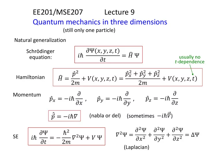
EE201/MSE207 Lecture 9 Quantum mechanics in three dimensions (still only one particle) Natural generalization 𝑗ℏ 𝜖Ψ(𝑦, 𝑧, 𝑨, 𝑢) Schrödinger = 𝐼 Ψ equation: usually no 𝜖𝑢 t -dependence 2 + 2 + 𝑞 2 2 2𝑛 + 𝑊 𝑦, 𝑧, 𝑨, 𝑢 = 𝑞 𝑦 𝑞 𝑧 𝑞 𝑨 𝐼 = + 𝑊 𝑦, 𝑧, 𝑨, 𝑢 Hamiltonian 2𝑛 𝑞 𝑨 = −𝑗ℏ 𝜖 𝑞 𝑦 = −𝑗ℏ 𝜖 𝑞 𝑧 = −𝑗ℏ 𝜖 Momentum 𝜖𝑦 , 𝜖𝑧 , 𝜖𝑨 (sometimes −𝑗ℏ𝛼 ) 𝑞 = −𝑗ℏ𝛼 (nabla or del) 𝛼 2 Ψ = 𝜖 2 Ψ 𝜖𝑦 2 + 𝜖 2 Ψ 𝜖𝑧 2 + 𝜖 2 Ψ 𝜖𝑢 = − ℏ 2 𝑗ℏ 𝜖Ψ 𝜖𝑨 2 = ΔΨ 2𝑛 𝛼 2 Ψ + 𝑊 Ψ SE (Laplacian)

TISE and general solution of SE If 𝑊(𝑦, 𝑧, 𝑨) (potential energy does not depend on time), then simplification − ℏ 2 2𝑛 𝛼 2 𝜔 𝑜 𝑠 + 𝑊 𝜔 𝑜 𝑠 = 𝐹 𝑜 𝜔 𝑜 𝑠 TISE 𝐼𝜔 𝑜 = 𝐹 𝑜 𝜔 𝑜 𝑠 = (𝑦, 𝑧, 𝑨) General solution of SE exp −𝑗 𝐹 𝑜 Ψ 𝑠, 𝑢 = 𝑑 𝑜 𝜔 𝑜 𝑠 ℏ 𝑢 𝑜 Normalization ∞ ∞ 𝑑 𝑜 2 = 1 Ψ 2 𝑒𝑦 𝑒𝑧 𝑒𝑨 = 1 𝜔 𝑜 2 𝑒𝑦 𝑒𝑧 𝑒𝑨 = 1 𝑜 −∞ −∞

Separation of variables in Cartesian coordinates (not in the textbook) Simplification if 𝑊 𝑠 = 𝑊 1 𝑦 + 𝑊 2 𝑧 + 𝑊 3 𝑨 ; then 3D TISE can be replaced with three 1D equations − ℏ 2 𝜖 2 𝜔 𝜖𝑦 2 + 𝜖 2 𝜔 𝜖𝑧 2 + 𝜖 2 𝜔 TISE + 𝑊 𝑠 𝜔 = 𝐹 𝜔 𝜖𝑨 2 2𝑛 𝜔 𝑠 = 𝜔 1 𝑦 𝜔 2 𝑧 𝜔 3 𝑨 Look for (assume) Divide TISE by 𝜔 , then 𝜖 2 𝜔 2 𝑧 𝜖 2 𝜔 1 𝑦 𝜖 2 𝜔 3 𝑨 − ℏ 2 𝜖𝑧 2 𝜖𝑦 2 𝜖𝑨 2 + + + 𝑊 1 𝑦 + 𝑊 2 𝑧 + 𝑊 3 (𝑨) = 𝐹 2𝑛 𝜔 1 𝑦 𝜔 2 𝑧 𝜔 3 𝑨 Then three equations, with 𝐹 = 𝐹 1 + 𝐹 2 + 𝐹 3 𝜖 2 𝜔 1 𝑦 − ℏ 2 𝜖𝑦 2 + 𝑊 1 𝑦 = 𝐹 1 and two similar equations for 𝑧 and 𝑨 2𝑛 𝜔 1 𝑦

Simplification if 𝑊 𝑠 = 𝑊 1 𝑦 + 𝑊 2 𝑧 + 𝑊 3 𝑨 (cont.) − ℏ 2 𝜖 2 𝜔 1 𝑦 Rewrite as usual + 𝑊 1 𝑦 𝜔 1 𝑦 = 𝐹 1 𝜔 1 𝑦 𝜖𝑦 2 2𝑛 − ℏ 2 𝜖 2 𝜔 2 𝑧 + 𝑊 2 𝑧 𝜔 2 𝑧 = 𝐹 2 𝜔 2 𝑧 𝜖𝑧 2 2𝑛 − ℏ 2 𝜖 2 𝜔 3 𝑨 + 𝑊 3 𝑨 𝜔 3 𝑨 = 𝐹 3 𝜔 3 𝑨 𝜖𝑨 2 2𝑛 𝐹 = 𝐹 1 + 𝐹 2 + 𝐹 3 𝜔 𝑠 = 𝜔 1 𝑦 𝜔 2 𝑧 𝜔 3 (𝑨) 𝜔 𝑙,𝑚,𝑛 𝑠 = 𝜔 1,𝑙 𝑦 𝜔 2,𝑚 𝑧 𝜔 3,𝑛 (𝑨) Each equation has many solutions 𝐹 = 𝐹 𝑦,𝑙 + 𝐹 𝑧,𝑚 + 𝐹 𝑨,𝑛 Energy (replaced 1,2,3 with 𝑦, 𝑧, 𝑨 ) General solution 𝑑 𝑙,𝑚,𝑛 𝜔 1,𝑙 𝑦 𝜔 2,𝑚 𝑧 𝜔 3,𝑛 (𝑨) exp −𝑗 𝐹 𝑦,𝑙 + 𝐹 𝑧,𝑚 + 𝐹 𝑨,𝑛 Ψ 𝑠, 𝑢 = 𝑢 ℏ 𝑙, 𝑚, 𝑛

Examples Unfortunately, not many examples when this trick is useful Semiconductor quantum well, quantum wire, quantum dot (terminology for semiconductor structures is slightly different than in QM) quantum well (QW), 2D electron gas (2DEG) z electrons do not move in z -direction, free motion in x and y quantum wire (QWi), 1D electrons electrons move only in x -direction, restricted along y and z x quantum dot (QD), 0D electrons motion is restricted in all direction ( x , y, and z) Only the first case (QW) can be truly represented as 𝑊 1 𝑦 + 𝑊 2 𝑧 + 𝑊 3 𝑨 ; however, other cases can also be treated in this way approximately

Semiconductor Quantum Well 𝑊 𝑠 = 𝑊 𝑨 = 0 + 0 + 𝑊 3 𝑨 z 𝑏 z (finite depth QW along z ) Wavefunctions 𝜔(𝑦, 𝑧, 𝑨) = 𝜔 𝑜 𝑨 𝑓 𝑗𝑙 𝑦 𝑦 𝑓 𝑗𝑙 𝑧 𝑧 1 2𝜌 or 1 2𝜌ℏ 𝐹 = 𝐹 𝑜 + ℏ 2 𝑙 𝑦 2𝑛 + ℏ 2 𝑙 𝑧 2 2 2𝑛 𝑠 = 0, 0 ≤ 𝑨 ≤ 𝑏 𝑊 then If infinite depth, ∞, otherwise 𝑜𝜌 𝑓 𝑗𝑙 𝑦 𝑦 𝑓 𝑗𝑙 𝑧 𝑧 1 2 𝑏 sin 𝜔(𝑦, 𝑧, 𝑨) = 𝑏 𝑨 or 1 2𝜌 2𝜌ℏ 2𝑛 + ℏ 2 𝑙 𝑧 2 𝐹 = 𝑜 2 𝜌 2 ℏ 2 2𝑛𝑏 2 + ℏ 2 𝑙 𝑦 2 a 0 2𝑛

Rectangular Quantum Wire 𝑐 If finite depth in y and z directions, then we cannot 𝑏 use this trick. However, it works for infinite depth. x if 0 ≤ 𝑨 ≤ 𝑏 𝑊 𝑦, 𝑧, 𝑨 = 0, 0 ≤ 𝑧 ≤ 𝑐 Assume ∞, otherwise 𝑏 𝑨 sin 𝑜 𝑧 𝜌 2 2 𝑐 sin 𝑜 𝑨 𝜌 1 𝑐 𝑧 𝑓 𝑗𝑙 𝑦 𝑦 𝜔 𝑦, 𝑧, 𝑨 = 𝑏 2𝜌 1 or 2 𝜌 2 ℏ 2 2 𝜌 2 ℏ 2 2𝜌ℏ 2𝑛𝑐 2 + ℏ 2 𝑙 𝑦 2 𝐹 = 𝑜 𝑨 2𝑛𝑏 2 + 𝑜 𝑧 2𝑛 If not rectangular and/or finite depth, then still 2+1 dimensions

Rectangular (cuboid) Quantum Dot 𝑐 Again need to assume infinite depth 𝑏 𝑑 0 ≤ 𝑨 ≤ 𝑏 0, if 0 ≤ 𝑧 ≤ 𝑐 𝑊 𝑦, 𝑧, 𝑨 = 0 ≤ 𝑦 ≤ 𝑑 ∞, otherwise 𝑏 𝑨 sin 𝑜 𝑧 𝜌 2 2 2 𝑑 sin 𝑜 𝑨 𝜌 𝑐 𝑧 sin 𝑜 𝑦 𝜌 𝜔 𝑦, 𝑧, 𝑨 = 𝑑 𝑦 𝑏 𝑐 2 2 2 𝜌 2 ℏ 2 𝑜 𝑨 𝑏 2 + 𝑜 𝑧 𝑐 2 + 𝑜 𝑦 𝐹 = 𝑑 2 2𝑛 Degeneracy if 𝑏 , 𝑐 , and 𝑑 are equal or commensurate. In semiconductors 𝑛 is effective mass.

Another example: 3D oscillator (e.g., atom in a lattice) 𝑠 = 1 2 𝑦 2 + 1 2 𝑧 2 + 1 2 𝑨 2 𝑊 2 𝑛𝜕 𝑦 2 𝑛𝜕 𝑧 2 𝑛𝜕 𝑨 1 1 2 ℏ𝜕 𝑧 + 𝑜 𝑨 + 1 𝐹 𝑜 𝑦 ,𝑜 𝑧 ,𝑜 𝑨 = 𝑜 𝑦 + 2 ℏ𝜕 𝑦 + 𝑜 𝑧 + 2 ℏ𝜕 𝑨 Again, degeneracy if 𝜕 𝑦 , 𝜕 𝑧 , or 𝜕 𝑨 are equal or commensurate.

Spherically symmetric potential (similar trick) 𝑊 𝑠 = 𝑊( 𝑠 ) Most important for atoms 𝜔 𝑠, 𝜄, 𝜒 = 𝑆 𝑠 𝑍(𝜄, 𝜒) Then it is natural to look for where 𝑠, 𝜄, 𝜒 are spherical coordinates − ℏ 2 2𝑛 𝛼 2 𝜔 + 𝑊 𝑠 𝜔 = 𝐹 𝜔 TISE Rewriting Laplacian in spherical coordinates − ℏ 2 𝜖 2 𝜔 1 𝜖𝑠 𝑠 2 𝜖𝜔 𝜖 1 𝜖𝜄 sin 𝜄 𝜖𝜔 𝜖 1 + + 𝜖𝜒 2 + 𝑊 𝑠 𝜔 = 𝐹 𝜔 𝑠 2 sin 𝜄 𝑠 2 sin 2 𝜄 𝑠 2 2𝑛 𝜖𝑠 𝜖𝜄 combine Divide by 𝜔 = 𝑆𝑍 and multiply by −2𝑛𝑠 2 /ℏ 2 − 2𝑛𝑠 2 𝜖 2 𝑍 1 𝜖𝑠 𝑠 2 𝜖𝑆 𝜖 + 1 1 𝜖𝜄 sin 𝜄 𝜖𝑍 𝜖 1 𝑊 𝑠 − 𝐹 + 𝜖𝜒 2 = 0 sin 2 𝜄 ℏ 2 𝑆 𝜖𝑠 𝑍 sin 𝜄 𝜖𝜄 const const 𝑚 (𝑚 + 1) −𝑚 (𝑚 + 1) (so far just a notation)

Spherical harmonics 𝑍 Assume 𝑍 𝜄, 𝜒 = Θ 𝜄 Φ(𝜒) , again separation of variables 𝜖 2 Φ 1 1 𝜖𝜄 sin 𝜄 𝜖Θ 𝜖 1 + 𝑚 𝑚 + 1 sin 2 𝜄 + 𝜖𝜒 2 = 0 Θ(𝜄) sin 𝜄 𝜖𝜄 Φ(𝜒) −𝑛 2 const 𝑛 2 const Φ 𝜒 = 𝑓 𝑗𝑛𝜒 , 𝑛 = 0, ±1, ±2, … (since should be periodic with 2𝜌) This is why 𝑛 is integer. 𝑛 (cos 𝜄) Θ 𝜄 = 𝐵 𝑄 𝑚 This is why 𝑚 is integer. Associated Legendre function 𝑚: anguar momentum quantum number 𝑚 = 0, 1, 2, … (integer) (azimuthal q. n. , orbital q. n. ) 𝑛 = −𝑚, −𝑚 + 1, … 0, … 𝑚 − 1, 𝑚 𝑛: magnetic quantum number 𝑛 𝜄, 𝜒 = Θ 𝑚 𝑛 𝜄 Φ 𝑛 (𝜒) 𝑍 are called spherical harmonics 𝑚 These function are the same for any spherically symmetric potential 𝑊(𝑠) .

Radial function 𝑆 𝜔 = 𝑆 𝑠 𝑍(𝜄, 𝜒) Let us introduce 𝑣 𝑠 = 𝑠 𝑆 𝑠 , for this function the equation is − ℏ 2 𝑒 2 𝑣 𝑒𝑠 2 + 𝑊 𝑠 + ℏ 2 𝑚 𝑚 + 1 𝑣 = 𝐹 𝑣 𝑠 2 2𝑛 2𝑛 centrifugal term So, the equation for 𝑣(𝑠) is similar to 1D TISE, but with the centrifugal term. It has some solutions, depending on 𝑚 (orbital q.n.) and 𝑜 (solution index). Corresponding energy: 𝐹 𝑜,𝑚 . Overall, 3 quantum numbers: 𝑜, 𝑚, 𝑛 . However, energy depends only on 𝑜 and 𝑚 .

Hydrogen atom 𝑊(𝑠) 𝑊 𝑠 = − 𝑓 2 1 4𝜌𝜁 0 𝑠 Consider only bound states (since atom)  𝐹 < 0 Effective potential − 𝑓 2 𝑠 + ℏ 2 1 𝑚 𝑚 + 1 𝑠 2 4𝜌𝜁 0 2𝑛 Accidentally, for this potential 𝐹 𝑜,𝑚 is highly degenerate 2 𝑓 2 𝑜 = 1, 2, 3, … 𝑛 𝑜 2 = 𝐹 1 1 𝐹 𝑜 = − 2ℏ 2 𝑜 2 4𝜌𝜁 0 𝐹 1 = −13.6 eV (ground state) 1 𝑜 = 1, 2, 3, … 𝜌𝑏 3 𝑓 −𝑠/𝑏 Ground state: 𝜔 100 𝑠, 𝜄, 𝜒 = principal 𝑚 = 0, 1, … 𝑜 − 1 azimuthal 𝑏 = 4𝜌𝜁 0 ℏ 2 (ang.mom.) 𝑛 = 0, ±1, ±2, … ± 𝑚 magnetic = 0.53 Å 𝑛𝑓 2 𝑜−1 (2𝑚 + 1) = 𝑜 2 Total degeneracy: 𝑚=0 Bohr radius (almost same theory for dopant levels and excitons)

Hydrogen atom (cont.) 𝜔 𝑜𝑚𝑛 𝑠, 𝜄, 𝜒 = 1 𝑠 𝜍 𝑚+1 𝑓 −𝜍 𝑤 𝜍 × 𝑍 𝑛 (𝜄, 𝜒) 𝑚 𝜍 = 𝑠 𝑏 = 4𝜌𝜁 0 ℏ 2 (Bohr radius, 0.53 ∙ 10 −10 m ) 𝑛𝑓 2 𝑏𝑜 𝑤 𝜍 is some polynomial of degree 𝑜 − 𝑚 − 1 (related to generalized Laguerre polynomial) Spectrum 2 1 2 − 1 𝑓 2 𝑛 1 ℏ𝜕 ph = 𝐹 𝑗 − 𝐹 𝑔 = −13.6 eV 𝐹 𝑜 = − 2 2ℏ 2 𝑜 2 𝑜 𝑗 𝑜 𝑔 4𝜌𝜁 0 … 5 4 Paschen series (infrared, 1908) 3 1 1 2 − 1 Balmer series (visible, 1885) Rydberg 𝜇 = 𝑆 2 2 𝑜 𝑔 𝑜 𝑗 formula, 1888 2 Lyman series (ultraviolet, 1906-14) 𝑓 2 𝑛 𝑆 = Rydberg constant 4𝜌𝑑ℏ 3 4𝜌𝜁 0 1.1 ∙ 10 7 m −1 1