
SLIDE 1
PCES 4.21
QUANTUM MECHANICS – Intro to Basic Features
- 1. QUANTUM INTERFERENCE & QUANTUM PATHS
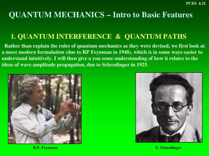
Rather than explain the rules of quantum mechanics as they were devised, we first look at a more modern formulation (due to RP Feynman in 1948), which is in some ways easier to understand intuitively. I will then give a you some understanding of how it relates to the ideas of wave amplitude propagation, due to Schrodinger in 1925.
R.P. Feynman
- E. Schrodinger