(quantum statistics) Classical statistical mechanics 1. - PowerPoint PPT Presentation

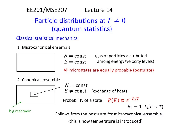
EE201/MSE207 Lecture 14 Particle distributions at 𝑈 ≠ 0 (quantum statistics) Classical statistical mechanics 1. Microcanonical ensemble 𝑂 = const (gas of particles distributed 𝐹 = const among energy/velocity levels) All microstates are equally probable (postulate) 2. Canonical ensemble 𝑂 = const 𝐹 ≠ const (exchange of heat) 𝑄 𝐹 ∝ 𝑓 −𝐹/𝑈 Probability of a state ( 𝑙 𝐶 = 1, 𝑙 𝐶 𝑈 → 𝑈 ) big reservoir Follows from the postulate for microcaconical ensemble (this is how temperature is introduced)

Classical statistical mechanics (cont.) 3. Grand canonical ensemble 𝑂 ≠ const (particles can penetrate) 𝐹 ≠ const Probability of a state 𝑄 𝐹, 𝑂 ∝ 𝑓 −(𝐹−𝜈𝑂)/𝑈 (two parameters: temperature and chemical potential) Chemical potential 𝜈 : average energy cost of bringing an extra particle from big reservoir The formula for 𝑄(𝐹, 𝑂) also follows from equiprobability in microcanonical ens. From 𝑄(𝐹, 𝑂) we can derive 𝑜(𝜁) : average number of particles with energy 𝜁 𝑜 𝜁 = exp − 𝜁 − 𝜈 𝐹 = 𝑗 𝑜 𝜁 𝑗 𝜁 𝑗 Maxwell-Boltzmann distribution 𝑈 𝑄 𝑙 : probability to have 𝑙 particles with quantized (binned) energy 𝜁 Derivation 𝑓 −𝑙 𝜁−𝜈 /𝑈 𝑙! ( 𝑙! comes from number of combinations) 𝑄 𝑙 = 𝑄 0  ∞ 𝑙=0  𝑄 0 = 𝑄 𝑙 = 1 1 exp[exp(−(𝜁 − 𝜈)/𝑈)] 𝑙 = exp[− (𝜁 − 𝜈) 𝑈]

Quantum statistics Main difference: indistinguishable particles (instead of a question “which one” we are only allowed to ask “how many”) 1 12 2 Example: two particles classical 12 2 1 on two levels equal probabilities, 1/4 each I II quantum II I equal probabilities, 1/3 each Fermions Either 0 or 1 particle on a level with energy 𝜁 (spin increases number of levels, still no 2 particles on the same level) 𝑄 1 = 𝑓 − 𝜁−𝜈 /𝑈 Still use classical relation 𝑄 𝐹, 𝑂 ∝ 𝑓 − 𝐹−𝜈𝑂 /𝑈 𝑄 0 1 𝑓 − 𝜁−𝜈 /𝑈 ⇒ 𝑄 0 = 1 + 𝑓 − 𝜁−𝜈 /𝑈 , 𝑄 1 = 1 + 𝑓 − 𝜁−𝜈 /𝑈 , 𝑄 0 + 𝑄 1 = 1 1 Fermi-Dirac distribution ⇒ 𝑜 = 𝑄 1 = (Fermi statistics) 1 + 𝑓 𝜁−𝜈 /𝑈 𝜈 is Fermi level (chemical vs. electrochemical)

Quantum statistics (cont.) Bosons 𝑄 𝑄 𝑄 2 1 3 = 𝑓 − 𝜁−𝜈 /𝑈 , = 𝑓 −2 𝜁−𝜈 /𝑈 , = 𝑓 −3 𝜁−𝜈 /𝑈 , . . . 𝑄 𝑄 𝑄 0 0 0 1 1 + 𝑓 − 𝜁−𝜈 /𝑈 + 𝑓 −2 𝜁−𝜈 /𝑈 + . . . = 1 − 𝑓 − 𝜁−𝜈 /𝑈 ⇒ 𝑄 𝑄 0 = 𝑜 = 1 1 + 2 ∙ 𝑄 2 + . . . = 1 − 𝑓 −𝜁−𝜈 (1 ∙ 𝑓 −𝜁−𝜈 𝑈 + 2 ∙ 𝑓 −2𝜁−𝜈 𝑈 + ⋯ ) 𝑜 = 0 ∙ 𝑄 0 + 1 ∙ 𝑄 𝑈 𝑓 −𝜁−𝜈 𝑓 −2𝜁−𝜈 𝑓 −𝜁−𝜈 = 1 − 𝑓 −𝜁−𝜈 𝑈 𝑈 𝑈 + + ⋯ = 𝑈 1 − 𝑓 −𝜁−𝜈 1 − 𝑓 −𝜁−𝜈 1 − 𝑓 −𝜁−𝜈 𝑈 𝑈 𝑈 1 Bose-Einstein distribution 𝑜 = 𝑓 𝜁−𝜈 /𝑈 − 1 (Bose statistics) 𝜈 ≤ 0 (if energy starts from 0), otherwise infinity at 𝜁 = 𝜈

Particle distributions: summary   𝑓 − 𝜁−𝜈 /𝑈 Maxwell-Boltzmann   𝜁 (Boltzmann) 1 𝑈 = 0  𝑜 𝜁 = Fermi-Dirac 𝑓 𝜁−𝜈 /𝑈 + 1  (Fermi)  𝜁 𝜈 1    Bose-Einstein 𝑓 𝜁−𝜈 /𝑈 − 1  (Bose)  𝜁 𝜈 𝜈 is Fermi level   To find 𝜈 : 𝑂 = 𝑜 𝜁 𝐸 𝜁 𝑒𝜁 𝑜(𝜁) depends on temperature ⇒ 𝜈 depends on temperature density of states Remark 1. Often notation 𝑔 𝜁 instead of 𝑜(𝜁) , especially for Fermi distribution Remark 2. Large- 𝜁 tails of Fermi-Dirac and Bose-Einstein distributions coincide with Maxwell-Boltzmann distribution

2D case (not in textbook) 𝐸 𝜁 𝑛 𝐸 𝜁 is density of states, 𝐵 is area = 2𝑡 + 1 2𝜌ℏ 2 𝐵 𝑡 is spin, in general 2𝑡 + 1 is degeneracy Electrons (Fermi, 𝑡 = 1 2 ) spin spin ∞ 𝑂 𝑛 1 𝑛 2𝜌ℏ 2 2 𝑈 ln(1 + 𝑓 𝜈/𝑈 ) 𝐵 = 2𝜌ℏ 2 2 𝑓 (𝜁−𝜈)/𝑈 + 1 𝑒𝜁 = 0 No spin factor of 2 in high magnetic field Bosons with 𝑡 = 0 ∞ 𝑂 𝑛 1 𝑛 2𝜌ℏ 2 𝑈 ln(1 − 𝑓 𝜈/𝑈 ) 𝐵 = 𝑓 (𝜁−𝜈)/𝑈 − 1 𝑒𝜁 = 2𝜌ℏ 2 0

3D case = 𝑛 3/2 𝜁 1/2 𝐸 𝜁 𝐸 𝜁 is density of states, 𝑊 is volume 2𝑡 + 1 𝑊 2 𝜌 2 ℏ 3 𝑡 is spin, in general 2𝑡 + 1 is degeneracy (including valleys, etc.) ∞ 𝑛 3/2 𝜁 1/2 𝑂 1 𝑊 = 𝑓 (𝜁−𝜈)/𝑈 ± 1 (2𝑡 + 1) 𝑒𝜁 2 𝜌 2 ℏ 3 0 degeneracy ∞ 𝜁 𝑛 3/2 𝜁 1/2 𝐹 1 𝑊 = 𝑓 (𝜁−𝜈)/𝑈 ± 1 (2𝑡 + 1) 𝑒𝜁 (e.g., for heat capacity) 2 𝜌 2 ℏ 3 0 Fermi: “ + ”, Bose: “ − ” Unfortunately, these integrals cannot be calculated analytically. Simplification if −𝜈 ≫ 𝑈 , then F-D and B-E distributions reduce to M-B. 1 𝑓 (𝜁−𝜈)/𝑈 ± 1 ≈ 𝑓 − 𝜁−𝜈 /𝑈 𝜁 − 𝜈 ≫ 𝑈 when

Nondegenerate semiconductor Assume n-type (p-type similar), −𝜈 ≫ 𝑈 , 2𝑡 + 1 = 2 conduction band > 3𝑈 𝜈 ∞ 𝑛 3/2 𝜁 1/2 (Fermi level) 𝑂 2 𝜌 2 ℏ 3 𝑓 −(𝜁−𝜈)/𝑈 2 𝑒𝜁 = . . . 𝑊 ≈ 0 valence band (neglect) 3/2 𝑛𝑈 = 2 𝑓 𝜈/𝑈 Room temperature: 𝑈 = 26 meV 2𝜌ℏ 2 3/2 2𝜌ℏ 2 𝜈 = 𝑈 ln 𝑂 1 𝑊 2 𝑛𝑈 degeneracy; can be larger, Si: 2  6 ∞ 𝜁 𝑛 3 2 𝜁 1 2 𝐹 𝑈 2 𝑒𝜁 = . . . = 3 2 𝑈 𝑂 2 𝜌 2 ℏ 3 𝑓 − 𝜁−𝜈 𝑊 ≈ 𝑊 0 𝐹 = 3 2 𝑈𝑂

Bose-Einstein condensation For Bose-Einstein distribution usually 𝜈 < 0 (cannot be 𝜈 > 0 ). However, at small enough 𝑈 , it becomes 𝜈 = 0 , then ∞ 𝑛 3/2 𝜁 1/2 3 𝑂 1 𝑛𝑈 ( 𝑡 = 0) 𝑊 = 𝑓 −𝜈/𝑈 − 1 𝑒𝜁 = 2.61 2𝜌ℏ 2 2 𝜌 2 ℏ 3 0 2/3 𝑑 = 2𝜌ℏ 2 𝑂 𝑈 Therefore critical temperature 𝑛 2.61 𝑊 Below 𝑈 𝑑 particles crowd into the ground state (finite fraction of all particles occupy ground state) 𝑂 = 𝑂 0 + 𝑜 𝜁 𝐸 𝜁 𝑒𝜁 Different calculation: Examples: superconductivity, superfluidity, B-E condensation of atoms

Massless particles (photons, phonons) 𝑙 = 2𝜌 𝜇 = 𝜕 𝜁 = ℏ𝜕 speed of light or sound velocity 𝑑 Number of particles is not conserved ⇒ 𝜈 = 0 (creation of extra particle does not cost extra energy) 1 𝑜(𝜕) = (bosons) 𝑓 ℏ𝜕/𝑈 − 1 𝑒𝑂 = 𝑒𝑦 𝑒𝑙 𝑦 𝑒𝑧 𝑒𝑙 𝑧 𝑒𝑨 𝑒𝑙 𝑨 𝑒𝑂 𝑊 = 𝑒𝑙 𝑦 𝑒𝑙 𝑧 𝑒𝑙 𝑨 ⇒ DOS: 2𝜌 3 2𝜌 3 𝑊 𝑒𝜕 = 4𝜌𝑙 2 𝜕 2 𝑒𝑂 𝑒𝑙 × 2 for photons (two polarizations) 𝑒𝜕 = 2 3 + 1 2𝜌 3 2𝜌 2 𝑑 3 × 3 for phonons, better 3 𝑑 ⊥ 𝑑 ∥ Average energy per d𝜕 (for photons) 𝑊 𝑒𝜕 = ℏ𝜕 2𝜕 2 2ℏ𝜕 3 𝑒𝐹 1 𝑓 ℏ𝜕/𝑈 − 1 = (Planck’s formula) 2𝜌 2 𝑑 3 (𝑓 ℏ𝜕/𝑈 − 1) 2𝜌 2 𝑑 3