Density matrix (density operator) In this course we described a - - PowerPoint PPT Presentation

EE201/MSE207 Lecture 18

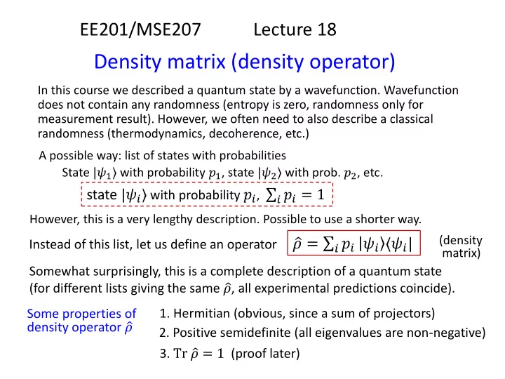
Density matrix (density operator)

In this course we described a quantum state by a wavefunction. Wavefunction does not contain any randomness (entropy is zero, randomness only for measurement result). However, we often need to also describe a classical randomness (thermodynamics, decoherence, etc.) (density matrix)

Instead of this list, let us define an operator

𝜍 = 𝑗 𝑞𝑗 𝜔𝑗 〈𝜔𝑗|

Somewhat surprisingly, this is a complete description of a quantum state (for different lists giving the same 𝜍, all experimental predictions coincide). Some properties of density operator 𝜍

However, this is a very lengthy description. Possible to use a shorter way. A possible way: list of states with probabilities State |𝜔1〉 with probability 𝑞1, state |𝜔2〉 with prob. 𝑞2, etc.

state |𝜔𝑗〉 with probability 𝑞𝑗, 𝑗 𝑞𝑗 = 1

• 1. Hermitian (obvious, since a sum of projectors)
• 2. Positive semidefinite (all eigenvalues are non-negative)
• 3. Tr

𝜍 = 1 (proof later)

For any observable 𝐵, its average (expectation) value is Theorem Proof

Averages via density matrix

for state |𝜔𝑗〉 with probability 𝑞𝑗, 𝑗 𝑞𝑗 = 1

𝜍 = 𝑗 𝑞𝑗 𝜔𝑗 〈𝜔𝑗| 𝐵 = Tr( 𝜍 𝐵)

(this is why 𝜍 is a complete description)

𝐵 = 𝑗 𝑞𝑗 〈𝜔𝑗 𝐵 𝜔𝑗〉 Tr 𝜍 𝐵 = 𝑙〈𝑓𝑙 𝜍 𝐵 𝑓𝑙〉

• rthonormal basis

Tr 𝜍 𝐵 = 𝑙〈𝑓𝑙 𝜍 𝐵 𝑓𝑙〉 = 𝑙,𝑗 𝑓𝑙 𝜔𝑗 𝑞𝑗 𝜔𝑗 𝐵 𝑓𝑙 =

𝜍

= 𝑗 𝑞𝑗 𝑙 𝜔𝑗 𝐵 𝑓𝑙 〈𝑓𝑙|𝜔𝑗〉 = 𝑗 𝑞𝑗 𝜔𝑗 𝐵 𝜔𝑗 = 〈 𝐵〉

1 QED Corollary

1 = Tr 𝜍 1 = Tr 𝜍

Therefore Tr

𝜍 = 1

Evolution of density matrix

𝜍 = 𝑗 𝑞𝑗 𝜔𝑗 〈𝜔𝑗|

𝑒 𝑒𝑢

𝜍 = 𝑗 𝑞𝑗

𝑒 𝜔𝑗 𝑒𝑢

𝜔𝑗 + |𝜔𝑗〉 𝑒 𝜔𝑗

𝑒𝑢

=

(Schrödinger equation for density matrix)

Tr 𝜍2 = 1 = − 𝑗

ℏ 𝑗 𝑞𝑗

𝐼 𝜔𝑗 〈𝜔𝑗| − |𝜔𝑗〉〈𝜔𝑗| 𝐼 = − 𝑗

ℏ

𝐼, 𝜍 𝑒 𝑒𝑢 𝜍 = − 𝑗 ℏ 𝐼, 𝜍 Pure and mixed states

Pure state: a state, which can be represented by a wavefunction |𝜔〉 with probability 𝑞 = 1, so

𝜍 = 𝜔 〈𝜔|

Then

𝜍2 = 𝜔 𝜔 𝜔 〈𝜔| = 𝜍

𝜍2 = 𝜍

Mixed state: a state, which can not be represented by a wavefunction Then

𝜍2 ≠ 𝜍 Tr 𝜍2 < 1 (proof via eigenbasis, 𝑞𝑗

2 < 𝑞𝑗 2 = 1)

Thermal distribution (equilibrium d.m.) 𝜍 = 𝑓−

𝐼/𝑈 Tr(𝑓− 𝐼/𝑈)

• r

𝜍 = 𝑓−(

𝐼−𝜈 𝑂)/𝑈 Tr(𝑓−( 𝐼−𝜈 𝑂)/𝑈)

In this case Schrödinger equation for state:

Next subject: Schrödinger and Heisenberg pictures

What we considered in this course is called Schrödinger picture. If 𝐼 is time-independent, then formally

Heisenberg picture 𝑒 𝑒𝑢 Ψ = − 𝑗 ℏ 𝐼|Ψ〉 Ψ(𝑢) = 𝑓−𝑗

𝐼𝑢/ℏ|Ψ(0)〉

Then expectation value of an observable 𝐵 at time 𝑢 is

𝐵 𝑢 = Ψ 𝑢 𝐵 Ψ 𝑢 = Ψ 0 𝑓𝑗

𝐼𝑢/ℏ

𝐵 𝑓−𝑗

𝐼𝑢/ℏ|Ψ(0)〉

We could get the same 〈 𝐵〉 is we assume that the state |Ψ〉 does not evolve, but instead the observable 𝐵 evolves with time 𝑢:

𝐵 𝑢 = 𝑓𝑗

𝐼𝑢/ℏ

𝐵 𝑓−𝑗

𝐼𝑢/ℏ

𝑒 𝑒𝑢 𝐵 𝑢 = 𝑗 ℏ 𝐼, 𝐵 𝑢

𝑒 𝑒𝑢 Ψ = 𝑗 𝐼0 ℏ 𝑓

𝑗 𝐼0𝑢 ℏ

Ψ + 𝑓

𝑗 𝐼0𝑢 ℏ

−𝑗 𝐼 ℏ Ψ = 𝑓

𝑗 𝐼0𝑢 ℏ

−𝑗 𝐼1 ℏ Ψ =

Interaction picture (main practical approach)

Interaction picture is a combination of both Schrödinger and Heisenberg pictures.

𝐼 = 𝐼0 + 𝐼1

Heisenberg-picture idea for 𝐼0. For any observable 𝐵, Also introduce

𝐵 𝑢 ≡ 𝑓𝑗

𝐼0𝑢/ℏ

𝐵 𝑓−𝑗

𝐼0𝑢/ℏ

𝑒 𝑒𝑢 𝐵 𝑢 = 𝑗 ℏ 𝐼0, 𝐵 𝑢

simple (solvable); assume time-independent

Ψ 𝑢 = 𝑓

𝑗 𝐼0𝑢 ℏ |Ψ 𝑢 〉

(here usual Schrödinger |Ψ 𝑢 〉) Then evolution for | Ψ 𝑢 〉 is So that

𝐵 𝑢 = Ψ 𝑢 𝐵 Ψ 𝑢 = Ψ 𝑢 𝑓

𝑗 𝐼0𝑢 ℏ

𝐵 𝑓

−𝑗 𝐼0𝑢 ℏ

| Ψ(𝑢)〉

𝐵 𝑢

SE

= 𝑓

𝑗 𝐼0𝑢 ℏ

−𝑗 𝐼1 ℏ 𝑓

−𝑗 𝐼0𝑢 ℏ

Ψ 𝑒 𝑒𝑢 Ψ = − 𝑗 ℏ 𝐼1 𝑢 Ψ

Heisenberg

Next subject: Methods for interacting electrons

(terminology and ideas)

Problem: 𝑊( 𝑠) changes because of electron-electron interaction, so need some self-consistent approach. 𝑊

0(

𝑠) “seed” potential

Thomas-Fermi method (or approximation)

Assume equilibrium Chemical potential 𝜈 (Fermi level) 𝜈 − 𝑊( 𝑠) Unknown 𝑊 𝑠 = 𝑊 𝑠 + Δ𝑊 𝑠 Idea: 𝜈 − 𝑊 𝑠 determines density of electrons, 𝑜(

𝑠) =

1 3𝜌2 2𝑛 𝜈−𝑊 ℏ2 3/2

, then solve Poisson equation to find Δ𝑊( 𝑠); self-consistency: 𝑊 → 𝑜 → 𝑊. Unknown 𝑊 𝑠 = 𝑊 𝑠 + Δ𝑊 𝑠

Hartree method (or approximation)

Non-equilibrium, but stationary case Idea: solve Schrödinger equation 𝐼𝜔 = 𝐹𝜔 to find 𝜔( 𝑠), then 𝑜 𝑠 ∝ 𝜔 𝑠

2,

then solve Poisson equation to find Δ𝑊( 𝑠); self-consistency 𝑊 → 𝜔 → 𝑜 → 𝑊. electron flow no chemical potential all electrons alike

Hartree-Fock method (or approximation)

Idea: almost the same as Hartree, but excludes e-e interaction for an electron with itself, so that electron feels only field produced by other electrons

Density functional theory

Even better (more accurate), uses functionals of electron density 𝑜( 𝑠) 𝑊 𝑠 = 𝑊 𝑠 + Δ𝑊 𝑠

Next subject: Language of second quantization

This is a technique to describe states with variable number of particles. (Later it was found to be useful for a fixed number of particles as well.) Occupation number representation

𝑂 = |𝑂1, 𝑂2, 𝑂3, … 〉

State with 𝑂1 particles on level 1, 𝑂2 particles

• n level 2, etc. We do not distinguish which

particle is where (indistinguishable). This is now the basis, so that an arbitrary (pure) state is a superposition:

𝜔 = 𝑂 𝑑(𝑂) 𝑂 𝑑 𝑂

2

is probability This wavefunction lives in the occupation number space (Fock space) Orthogonality:

〈𝑂 𝑂 = 1 〈𝑁 𝑂 = 0 if 𝑁 ≠ 𝑂,

Examples of (basis) states |0, 0, 0, … 〉 no particles, “vacuum”, |0〉 or |0〉 |0, 1, 0, … 〉

• ne particles in state 2

|0, 2, 1, 0, … 〉 two particles in state 2, 1 particle in state 3

Second quantization (cont.)

Simple special case: one oscillator (main language in optics) (Fock-space representation) Wavefunction: 𝜔 = 𝑜 𝑑 𝑜 |𝑜〉 Basis: 0 , |1〉, |2〉, |3〉, etc. Instead of the level number, we think about number of photons 𝑏2

† 0 = |0, 1, 0, 0, … 〉

Creation and annihilation operators 𝑏3

† 0 = |0, 0, 1, 0, … 〉

For bosons 𝑏𝑙

† … 𝑂𝑙, … =

𝑂𝑙 + 1 | … 𝑂𝑙 + 1, … 〉 creates extra particle on level 𝑙 (factor 𝑂 + 1 as for an oscillator) For bosons 𝑏𝑙 … 𝑂𝑙, … = 𝑂𝑙 | … 𝑂𝑙 − 1, … 〉 annihilates (kills) one particle on level 𝑙 (factor 𝑂 as for an oscillator) If 𝑂𝑙 = 0, then 𝑏𝑙 … 0𝑙, … = 0 (zero, not vacuum) In particular, 𝑏𝑙

†

𝑏𝑙 … 𝑂𝑙, … = 𝑂𝑙 | … 𝑂𝑙, … 〉, so 𝑂𝑙 = 𝑏𝑙

†

𝑏𝑙 Commutation relations

𝑏𝑙, 𝑏𝑚

† = 𝜀𝑙𝑚 ,

𝑏𝑙, 𝑏𝑚 = 𝑏𝑙

†,

𝑏𝑚

† = 0

Sufficient for the whole theory

Second quantization (cont.)

Operators can often be expressed in terms of 𝑏† and 𝑏

H = 𝑙 𝜁𝑙 𝑏𝑙

†

𝑏𝑙

If basis vectors are not eigenstates, then also terms 𝑙𝑚 𝐼𝑙𝑚

𝑏𝑙

†

𝑏𝑚

For fermions similar, but commutation relations are

𝑏𝑙, 𝑏𝑚

† + = 𝜀𝑙𝑚 ,

𝑏𝑙, 𝑏𝑚 + = { 𝑏𝑙

†,

𝑏𝑚

†}+ = 0

where 𝐵, 𝐶 + ≡ 𝐵 𝐶 + 𝐶 𝐵 (non-interacting particles, basis of eigenstates) Tight-binding model:

𝐼 = 𝑘 𝜁𝑘 𝑏𝑘

†𝑏𝑘 + 𝑘 (𝑈 𝑘𝑏𝑘 †𝑏𝑘+1 + 𝑈 𝑘 ∗𝑏𝑘+1 †

𝑏𝑘)

Coulomb interaction:

𝐼 = 𝑙𝑚 𝐼𝑙𝑚 𝑏𝑙

†

𝑏𝑙 𝑏𝑚

†

𝑏𝑚

For example, this means that 𝑏𝑙

†

𝑏𝑙

† 0 = −

𝑏𝑙

†

𝑏𝑙

† 0 , so

𝑏𝑙

†

𝑏𝑙

† 0 = 0

(Pauli exclusion principle) For one particle it does not matter if it is fermion or boson, so boson rules are often used for electrons (in single-particle approaches) Why called “second quantization”? 𝜔 𝑦 → 𝜔 = 𝑙 𝜔𝑙 𝑏𝑙