EE201/MSE207 Lecture 5 Bound and scattering (unbound) states - - PowerPoint PPT Presentation

EE201/MSE207 Lecture 5 Bound and “scattering” (unbound) states

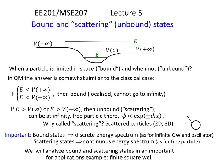
When a particle is limited in space (“bound”) and when not (“unbound”)? 𝑊 −∞ 𝑊 +∞ 𝐹 𝐹 𝑊 𝑦 In QM the answer is somewhat similar to the classical case: If 𝐹 < 𝑊(+∞) 𝐹 < 𝑊(−∞) , then bound (localized, cannot go to infinity) If 𝐹 > 𝑊 ∞ or 𝐹 > 𝑊 −∞ , then unbound (“scattering”); can be at infinity, free particle there, 𝜔 ∝ exp ±𝑗𝑙𝑦 . Why called “scattering”? Scattered particles (2D, 3D). Important: Bound states  discrete energy spectrum (as for infinite QW and oscillator) Scattering states  continuous energy spectrum (as for free particle) We will analyze bound and scattering states in an important for applications example: finite square well

Finite square well

− ℏ2 2𝑛 𝑒2𝜔 𝑒𝑦2 + 𝑊(𝑦)𝜔 = 𝐹𝜔

width 2𝑏 (it was 𝑏 for infinite well) depth 𝑊 Three regions: (1) 𝑦 < −𝑏, (2) −𝑏 < 𝑦 < 𝑏, (3) 𝑦 > 𝑏 𝑊(𝑦) 𝑏 −𝑏 −𝑊

𝑊 𝑦 = −𝑊

0 ,

−𝑏 < 𝑦 < 𝑏 0 , 𝑦 > 𝑏

Today: Bound states, 𝐹 < 0 (𝐹 < 𝐹 ±∞ = 0)

TISE 𝐹 −𝑊 𝐹 + 𝑊

𝐹 < 0 𝑊

0 > 0

𝐹 + 𝑊

0 > 0

(1) (2) (3)

− ℏ2 2𝑛 𝑒2𝜔 𝑒𝑦2 + 𝑊(𝑦)𝜔 = 𝐹𝜔

𝐵 = 0 because 𝜔 −∞ = 0

Solving TISE in 3 regions

𝐹 −𝑊 𝐹 + 𝑊

𝐹 < 0, 𝑊

0 > 0,

𝐹 + 𝑊

0 > 0

(1) (2) (3) (1) 𝑦 < −𝑏  𝑊 = 0 

𝑒2𝜔 𝑒𝑦2 = − 2𝑛𝐹 ℏ2 𝜔

> 0, = 𝑙2

𝜔 𝑦 = 𝐵 𝑓−𝑙𝑦 + 𝐶 𝑓𝑙𝑦, 𝑙 = −2𝑛𝐹 ℏ

(2) −𝑏 < 𝑦 < 𝑏  𝑊 = −𝑊 

𝑒2𝜔 𝑒𝑦2 = − 2𝑛(𝑊

0 + 𝐹)

ℏ2 𝜔

< 0, = −𝑚2

𝜔 𝑦 = 𝐷 sin(𝑚𝑦) + 𝐸 cos(𝑚𝑦) 𝑚 = 2𝑛(𝑊

0 + 𝐹)

ℏ

(sin and cos are more convenient for bound states,

𝑓±𝑗𝑚𝑦 more convenient for scattering states) (3) 𝑦 > 𝑏  𝑊 = 0 

𝜔 𝑦 = 𝐺 𝑓−𝑙𝑦 + 𝐻 𝑓𝑙𝑦

(the same 𝑙) 𝐻 = 0 because 𝜔 +∞ = 0

𝐹 −𝑊 𝐹 + 𝑊 (1) (2) (3) (1) 𝑦 < −𝑏

𝜔 𝑦 = 𝐶 𝑓𝑙𝑦, 𝑙 = −2𝑛𝐹 ℏ

(2) −𝑏 < 𝑦 < 𝑏

𝜔 𝑦 = 𝐷 sin(𝑚𝑦) + 𝐸 cos(𝑚𝑦) 𝑚 = 2𝑛(𝑊

0 + 𝐹) ℏ

(3) 𝑦 > 𝑏

𝜔 𝑦 = 𝐺 𝑓−𝑙𝑦

Boundary conditions:

1) 𝜔 𝑦 is continuous 2) 𝑒𝜔/𝑒𝑦 is also continuous 2’) actually, in semiconductors condition 2) is different:

1 𝑛𝑓𝑔𝑔 𝑒𝜔 𝑒𝑦 is continuous

(this is not discussed in Griffiths’ book) Follows from continuity

• f probability current

𝑗ℏ 2𝑛 𝜔 𝑒𝜔∗ 𝑒𝑦 − 𝜔∗ 𝑒𝜔 𝑒𝑦 We have 5 equations (4 boundary conditions and normalization) and 5 unknowns (𝐶, 𝐷, 𝐸, 𝐺, and 𝐹). Possible to solve, but too many. Simplification: trick of odd and even functions 𝑔 −𝑦 = 𝑔(𝑦) even 𝑔 −𝑦 = −𝑔(𝑦) odd

Trick of odd and even functions for even potential, 𝑊 −𝑦 = 𝑊(𝑦)

In our case 𝑊(𝑦) is even Theorem If 𝑊 −𝑦 = 𝑊(𝑦) and 𝜔 𝑦 is a solution of TISE with energy 𝐹, 𝐼𝜔 = 𝐹𝜔, then 𝜔(−𝑦) is also a solution with the same energy, 𝐼𝜔(−𝑦) = 𝐹𝜔(−𝑦). (simple to prove, and also quite obvious) Then 𝜔 𝑦 + 𝜔(−𝑦) is also a solution, and 𝜔 𝑦 − 𝜔(−𝑦) is also a solution (because TISE is linear in 𝜔), (not necessarily normalized, but not a problem) 𝜔 𝑦 + 𝜔(−𝑦) is even 𝜔 𝑦 − 𝜔(−𝑦) is odd (actually, if 𝜔(𝑦) is even or odd, then one of the combinations is zero) Therefore, it is sufficient to find only even and odd solutions of TISE

Even solutions for finite square well

𝜔 𝑦 = 𝐶 exp 𝑙𝑦 , 𝑦 < −𝑏 𝐸 cos 𝑚𝑦 , 𝑦 < 𝑏 𝐶 exp −𝑙𝑦 , 𝑦 > 𝑏

(no sin-term) (the same factor 𝐶)

• nly 3 unknowns:

𝐶, 𝐸, 𝐹 Boundary condition at 𝑦 = 𝑏 (b.c. at 𝑦 = −𝑏 gives the same): 𝐶 exp(−𝑙𝑏) = 𝐸 cos(𝑚𝑏) −𝑙𝐶 exp −𝑙𝑏 = −𝑚𝐸 sin(𝑚𝑏) Divide equations:

𝑙 = 𝑚 tan(𝑚𝑏)

This equation gives energy 𝐹 since 𝑙(𝐹), 𝑚(𝐹)

Rewrite: tan(𝑚𝑏) = 𝑙 𝑚 = −2𝑛𝐹/ℏ 2𝑛 𝑊

0 + 𝐹 /ℏ

= −𝐹 𝑊

0 + 𝐹 =

𝑊 𝑊

0 + 𝐹 − 1 =

𝑊

02𝑛

𝑚2ℏ2 − 1 tan(𝑚𝑏) = 𝑏2𝑊

02𝑛

ℏ2 𝑚𝑏 2 − 1

Even solutions for finite square well

tan(𝑚𝑏) = 𝑏2𝑊

02𝑛

ℏ2 𝑚𝑏 2 − 1 Solve graphically Finite number of solutions: 𝑂even = int 𝑏 ℏ 2𝑛𝑊 𝜌 + 1 Limiting cases 1) 𝑏2𝑊

02𝑛

ℏ2 ≫ 1 (wide, deep well) Low levels: 𝑚𝑏 ≈ 2𝑜 + 1 𝜌/2, 𝐹𝑜 + 𝑊

0 = 𝑚2ℏ2

2𝑛 ≈ 2𝑜 + 1 2𝜌2ℏ2 2𝑛 2𝑏 2 (similar to infinite well, but only odd states and 𝑏 → 2𝑏) 𝑏2𝑊

02𝑛

ℏ2 ≪ 1

2)

(shallow, narrow well) Only one level: 𝑚𝑏 ≈ 𝑏 2𝑛𝑊

0/ℏ ≪ 1,

𝐹 ≪ 𝑊 𝑚 = 2𝑛(𝑊

0 + 𝐹)

ℏ

Even solutions for finite square well: normalization

(not important)

−∞ ∞

𝜔 𝑦

2 𝑒𝑦 = 1

⟹ 𝜔 𝑦 = 𝐶 exp 𝑙𝑦 , 𝑦 < −𝑏 𝐸 cos 𝑚𝑦 , 𝑦 < 𝑏 𝐶 exp −𝑙𝑦 , 𝑦 > 𝑏

Normalization

𝐶 = exp 𝑙𝑏 cos(𝑚𝑏) 𝑏 + 1/𝑙 𝐸 = 1 𝑏 + 1/𝑙

Odd solutions (similar)

𝜔 𝑦 = 𝐶 exp 𝑙𝑦 , 𝑦 < −𝑏 𝐷 sin(𝑚𝑦), 𝑦 < 𝑏 −𝐶 exp −𝑙𝑦 , 𝑦 > 𝑏

(no cos-term) (−𝐶 since odd)

Boundary condition at 𝑦 = 𝑏: −𝐶 exp −𝑙𝑏 = 𝐷 sin(𝑚𝑏) 𝑙𝐶 exp −𝑙𝑏 = 𝐷𝑚 cos(𝑚𝑏) Divide equations:

𝑙 = −𝑚 cot(𝑚𝑏)

−cot(𝑚𝑏) = 𝑏2𝑊

02𝑛

ℏ2 𝑚𝑏 2 − 1 After some algebra: Similar to the even case, the only difference: tan 𝑚𝑏 → −cot(𝑚𝑏) (just shifted by 𝜌/2)

Odd solutions for finite square well

−cot(𝑚𝑏) = 𝑏2𝑊

02𝑛

ℏ2 𝑚𝑏 2 − 1 Number of solutions: 𝑂odd = int 𝑏 ℏ 2𝑛𝑊 𝜌 + 1 2 Limiting cases 1) 𝑏2𝑊

02𝑛

ℏ2 ≫ 1 (wide, deep well) Low levels: 𝑚𝑏 ≈ 𝑜𝜌, 𝐹𝑜 + 𝑊

0 = 𝑚2ℏ2

2𝑛 ≈ 2𝑜 2𝜌2ℏ2 2𝑛 2𝑏 2 (these are remaining solutions for infinite well with 𝑏 → 2𝑏)

2)

Shallow, narrow well No odd solutions if

Total number of solutions:

𝑂even + 𝑂odd = int 𝑏 ℏ 2𝑛𝑊 𝜌/2 + 1 𝑊

0 < 𝜌2ℏ2

8𝑛𝑏2

Digression: some integrals

−∞ ∞

𝑓−𝑏𝑦2𝑒𝑦 = 𝜌 𝑏

(easy to derive by squaring and considering as a double-integral; also from normalization of a Gaussian:

−∞ ∞ 1 2𝜌𝐸 𝑓−𝑦2/2𝐸𝑒𝑦 = 1.

Take derivative in respect to parameter 𝑏

−∞ ∞

−𝑦2 𝑓−𝑏𝑦2𝑒𝑦 = − 𝜌 2𝑏3/2

⇒

−∞ ∞

𝑦2 𝑓−𝑏𝑦2𝑒𝑦 = 𝜌 2𝑏3/2

Take another derivative with respect to 𝑏, similarly:

−∞ ∞

𝑦4 𝑓−𝑏𝑦2𝑒𝑦 = 3 𝜌 4𝑏5/2

(and so on: 𝑦6, 𝑦8, etc.) Can construct a similar series, starting with

∞

𝑦 𝑓−𝑏𝑦2𝑒𝑦 = 1 2𝑏