SLIDE 1
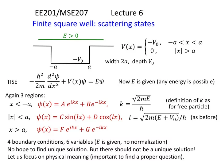
EE201/MSE207 Lecture 6 Finite square well: scattering states
width 2𝑏, depth 𝑊 𝑏 −𝑏 −𝑊
𝑊 𝑦 = −𝑊
0 ,
−𝑏 < 𝑦 < 𝑏 0 , 𝑦 > 𝑏
𝐹 > 0 TISE
− ℏ2 2𝑛 𝑒2𝜔 𝑒𝑦2 + 𝑊(𝑦)𝜔 = 𝐹𝜔
Now 𝐹 is given (any energy is possible) Again 3 regions:
𝑦 < −𝑏, 𝑙 = 2𝑛𝐹 ℏ
(definition of 𝑙 as for free particle)
𝑦 < 𝑏, 𝜔 𝑦 = 𝐷 sin(𝑚𝑦) + 𝐸 cos(𝑚𝑦), 𝑚 = 2𝑛 𝐹 + 𝑊
0 /ℏ (as before)
𝑦 > 𝑏,
4 boundary conditions, 6 variables (𝐹 is given, no normalization) No hope to find unique solution. But there should not be a unique solution! Let us focus on physical meaning (important to find a proper question).
𝜔 𝑦 = 𝐵 𝑓𝑗𝑙𝑦 + 𝐶𝑓−𝑗𝑙𝑦, 𝜔 𝑦 = 𝐺 𝑓𝑗𝑙𝑦 + 𝐻 𝑓−𝑗𝑙𝑦
SLIDE 2 Add time dependence
𝑦 < −𝑏, Ψ 𝑦, 𝑢 = 𝐵 𝑓
𝑗𝑙 𝑦 − ℏ𝑙 2𝑛 𝑢 + 𝐶 𝑓 −𝑗𝑙 𝑦 + ℏ𝑙 2𝑛 𝑢
incident wave
(as for free particle; different phase and group velocities, but the same direction)
𝐵 𝐶 Similarly for 𝑦 > 𝑏 𝐵 𝐶 𝐺 𝐻
(if necessary, wave packets can be constructed later; in reality nobody usually does it because it is too complicated; instead, people work with unnormalized states)
Assume that the wave is incident from the left, then 𝐻 = 0 𝐵 𝐶 𝐺 𝐵 is incident wave amplitude 𝐶 is reflected wave amplitude 𝐺 is transmitted wave amplitude We have 5 variables (𝐵, 𝐶, 𝐷, 𝐸, 𝐺) and 4 equations. Equations are linear. Can express 𝐶, 𝐷, 𝐸, 𝐺 as functions of 𝐵 (incident amplitude).
SLIDE 3
𝐵 𝐶 𝐺 𝐵 is incident wave amplitude 𝐶 is reflected wave amplitude 𝐺 is transmitted wave amplitude
Proper questions
Goal: find ratios 𝑠 = 𝐶
𝐵
and 𝑢 = 𝐺
𝐵
(these ratios are called reflection and transmission amplitudes)
(assume a wave incident from the left)
Reflection coefficient (probability of reflection)
𝑆 = 𝑠 2 = 𝐶 2 𝐵 2
Transmission coefficient (probability of transmission)
𝑈 = 𝑢 2 = 𝐺 2 𝐵 2
From physical meaning
𝑈 + 𝑆 = 1
Remark 1. Definition of 𝑈 is sometimes different (discuss later, × 𝑤𝑠/𝑤𝑚) Remark 2. Terminology: Reflection/transmission amplitudes (𝑠, 𝑢) and coefficients (𝑆, 𝑈) Remark 3. We defined 𝑆 and 𝑈 as ratios; they become probabilities for wave packets (possible to show). Quadratic because probability ∝ Ψ 2.
SLIDE 4
𝐵 𝐶 𝐺
Finding 𝑈 and 𝑆
Boundary conditions: Simple to exclude 𝐷 and 𝐸 (similar combinations), then 2 equations with 𝐵, 𝐶, 𝐺
𝑦 < −𝑏, 𝜔 𝑦 = 𝐵 𝑓𝑗𝑙𝑦 + 𝐶 𝑓−𝑗𝑙𝑦 𝑦 < 𝑏, 𝜔 𝑦 = 𝐷 sin(𝑚𝑦) + 𝐸 cos(𝑚𝑦) 𝑦 > 𝑏, 𝜔 𝑦 = 𝐺 𝑓𝑗𝑙𝑦
𝑗𝑙 𝐵 𝑓−𝑗𝑙𝑏 − 𝐶𝑓𝑗𝑙𝑏 = 𝑚 [𝐷 cos 𝑚𝑏 + 𝐸 sin 𝑚𝑏 ] 𝐷 sin 𝑚𝑏 + 𝐸 cos 𝑚𝑏 = 𝐺 𝑓𝑗𝑙𝑏 𝐵 𝑓−𝑗𝑙𝑏 + 𝐶𝑓𝑗𝑙𝑏 = −𝐷 sin 𝑚𝑏 + 𝐸 cos 𝑚𝑏 𝑚 [𝐷 cos 𝑚𝑏 − 𝐸 sin 𝑚𝑏 = 𝑗𝑙 𝐺 𝑓𝑗𝑙𝑏
𝑦 = −𝑏 𝑦 = 𝑏
Finally 𝐺 = 𝑓−2𝑗𝑙𝑏 cos 2𝑚𝑏 − 𝑗 sin 2𝑚𝑏 2𝑙𝑚 (𝑙2 + 𝑚2) 𝐵 𝐶 = 𝑗 sin 2𝑚𝑏 2𝑙𝑚 (𝑚2 − 𝑙2) 𝐺 𝑙 = 2𝑛𝐹 ℏ 𝑚 = 2𝑛 𝐹 + 𝑊 ℏ
SLIDE 5 𝐵 𝐶 𝐺
Finding 𝑈 and 𝑆
𝑦 < −𝑏, 𝜔 𝑦 = 𝐵 𝑓𝑗𝑙𝑦 + 𝐶 𝑓−𝑗𝑙𝑦 𝑦 > 𝑏, 𝜔 𝑦 = 𝐺 𝑓𝑗𝑙𝑦
𝑈 = 𝐺 2 𝐵 2 = 1 1 + 𝑊
2
4𝐹(𝐹 + 𝑊
0) sin2 2𝑏
ℏ 2𝑛 𝐹 + 𝑊 Transmission probability
−𝑊 𝐹
Reflection probability 𝑆 = 1 − 𝑈 (too long from 𝐶 2/ 𝐵 2)
2𝑏 ℏ 2𝑛(𝐹 + 𝑊
0) = 𝑜𝜌
⟺ 𝐹 + 𝑊
0 = 𝑜2𝜌2ℏ2
2𝑛 2𝑏 2 This is exactly the “simple” energy quantization (in infinite well). Explanation: destructive interference of reflected waves (similar to anti-reflective coating with quarter-wavelength films).
SLIDE 6
𝐶 𝐻 𝐺
Now wave incident from the right
𝑦 < −𝑏, 𝜔 𝑦 = 𝐶 𝑓−𝑗𝑙𝑦 𝑦 > 𝑏, 𝜔 𝑦 = 𝐺 𝑓𝑗𝑙𝑦 + 𝐻 𝑓−𝑗𝑙𝑦
−𝑊 𝐹
𝑈
r = 𝑢r 2 = 𝐶 2
𝐻 2 Similarly, we can find transmission and reflection coefficients In our case because of symmetry However, this is always true (for any potential 𝑊 𝑦 and possibly different masses) 𝑆r = 𝑠
r 2 = 𝐺 2
𝐻 2 𝑈
r + 𝑆r = 1
𝑈
r = 𝑈 l = 𝑈
𝑆r = 𝑈
l = 𝑆
SLIDE 7
𝑈 and 𝑆 in general case
Why? Probability current If 𝜔 𝑦 = 𝐵 𝑓𝑗𝑙𝑦, then 𝑆 = 𝐶 2 𝐵 2 = 𝑠 2 𝑊 −∞ 𝑊 +∞ 𝐹 𝑊 𝑦 𝑊 −∞ ≠ 𝑊 ∞ and/or 𝑛1 ≠ 𝑛2
𝑛1 𝑛2 𝐵 𝐶 𝐺
𝑈 = 𝐺 2 𝐵 2 𝐹 − 𝑊(+∞) 𝐹 − 𝑊(−∞) 𝑛1 𝑛2 = 𝐺 2 𝐵 2 𝑙2/𝑛2 𝑙1/𝑛1 = 𝐺 2 𝐵 2 𝑤2 𝑤1 = 𝑢 2 𝑤2 𝑤1 𝑈 + 𝑆 = 1 𝐾 = 𝑗ℏ 2𝑛 𝜔 𝑒𝜔∗ 𝑒𝑦 − 𝜔∗ 𝑒𝜔 𝑒𝑦 𝐾 = 𝐵 2 ℏ𝑙 𝑛 = 𝐵 2𝑤
(remember that 𝑛−1 𝑒𝜔
𝑒𝑦 is
continuous, not just
𝑒𝜔 𝑒𝑦)
The same velocity for reflection, but may be different for transmission
SLIDE 8
Transmission/reflection for -potential
𝐵 𝑓𝑗𝑙𝑦 𝐺 𝑓𝑗𝑙𝑦 𝐶 𝑓−𝑗𝑙𝑦 𝐻 𝑓−𝑗𝑙𝑦 𝑊 𝑦 = 𝛽 𝜀 𝑦
TISE
− ℏ2 2𝑛 𝑒2𝜔 𝑒𝑦2 + 𝑊(𝑦)𝜔 = 𝐹𝜔
𝐹 > 0 Integrate TISE near zero,
− ℏ2 2𝑛 𝜔′ 𝜁 − 𝜔′ −𝜁 + 𝛽 𝜔(0) = 0
−𝜁 𝜁
… ⇒
𝜁 → 0
𝑒𝜔(+0) 𝑒𝑦 − 𝑒𝜔 −0 𝑒𝑦 = 2𝑛𝛽 ℏ2 𝜔(0)
With -potential, 𝑒𝜔/𝑒𝑦 has a step (not continuous). Boundary conditions 𝐵 + 𝐶 = 𝐺 + 𝐻 𝑗𝑙 𝐺 − 𝐻 − 𝑗𝑙(𝐵 − 𝐶) = 2𝑛𝛽 ℏ2 (𝐵 + 𝐶) If 𝐻 = 0 (incident from the left), then 𝐶 𝐵 = −𝑗 𝑛𝛽 ℏ2𝑙 1 + 𝑗 𝑛𝛽 ℏ2𝑙 , 𝐺 𝐵 = 1 1 + 𝑗 𝑛𝛽 ℏ2𝑙
𝑙 = 2𝑛𝐹/ℏ
𝛽 𝜀 𝑦
SLIDE 9
Scattering matrix (now waves incident from both sides)
Suppose we found transmission/reflection amplitudes (𝑢𝑚, 𝑠
𝑚) for the wave
incident from the left and also from the right (𝑢𝑠, 𝑠
𝑠).
It is convenient to write these 4 complex numbers as a 2 × 2 matrix. For simplicity assume 𝑊 −∞ = 𝑊 ∞ , 𝑛1 = 𝑛2 𝑦 → −∞ Out of 4 wave amplitudes (𝐵, 𝐶, 𝐺, 𝐻), 2 free parameters, and the other 2 can be calculated (linear relations) 𝑊 𝑦
𝐵 𝐶 𝐺 𝐻
𝑦 → ∞ 𝜔 𝑦 = 𝐵𝑓𝑗𝑙𝑦 + 𝐶𝑓−𝑗𝑙𝑦 𝜔 𝑦 = 𝐺𝑓𝑗𝑙𝑦 + 𝐻𝑓−𝑗𝑙𝑦 Why 2 free parameters? 1) it was 2 in rectangular well 2) TISE is a second-order dif. eq. 2 boundary conditions
𝑇 = 𝑠
𝑚
𝑢𝑠 𝑢𝑚 𝑠
𝑠
= 𝑇11 𝑇12 𝑇21 𝑇22
What is the meaning? (scattering matrix)
𝐶 𝐺 = 𝑇 𝐵 𝐻
(outgoing via incoming)
[not included into this course]
SLIDE 10
Scattering matrix (S-matrix)
For simplicity assume 𝑊 −∞ = 𝑊 ∞ , 𝑛1 = 𝑛2 𝑦 → −∞ 𝑊 𝑦
𝐵 𝐶 𝐺 𝐻
𝑦 → ∞ 𝜔 𝑦 = 𝐵𝑓𝑗𝑙𝑦 + 𝐶𝑓−𝑗𝑙𝑦 𝜔 𝑦 = 𝐺𝑓𝑗𝑙𝑦 + 𝐻𝑓−𝑗𝑙𝑦
𝑇 = 𝑠
𝑚
𝑢𝑠 𝑢𝑚 𝑠
𝑠
= 𝑇11 𝑇12 𝑇21 𝑇22
What is the meaning?
𝐶 𝐺 = 𝑇 𝐵 𝐻
(outgoing via incoming) Suppose 𝐻 = 0, then
𝐶 𝐺 = 𝑠
𝑚 𝐵
𝑢𝑚𝐵
Suppose A = 0, then
𝐶 𝐺 = 𝑢𝑠 𝐻 𝑠
𝑠𝐻
𝑈
𝑚 = 𝑢𝑚 2 = 𝑇21 2, 𝑆𝑚 = 𝑠 𝑚 2 = 𝑇11 2
𝑈
𝑠 = 𝑢𝑠 2 = 𝑇12 2, 𝑆𝑠 = 𝑠 𝑠 2 = 𝑇22 2
(remember that formulas for 𝑈 in general case are different)
Let us prove symmetry:
𝑆𝑚 = 𝑆𝑠 𝑈𝑚 = 𝑈
𝑠
(for brevity will use notation: 𝑢𝑚 = 𝑢, 𝑠
𝑚 = 𝑠)
SLIDE 11
Symmetry of the scattering matrix
Our proof will use “graphical operations” with solutions of TISE
𝐵 = 1 𝑠 𝑢
TISE
Conjugate solution of TISE 𝑠∗ 1 𝑢∗ × −1 𝑠∗
+
𝑠 − 1 𝑠∗ 𝑢 − 𝑢∗ 𝑠∗ Now multiply by
−𝑠∗ 𝑢∗
−𝑠∗ 𝑢∗ 𝑠 − 1 𝑠∗ =
−𝑠∗ 𝑢 𝑢∗ 1
= 1 − |𝑠|2 𝑢∗ = 𝑢 2 𝑢∗ = 𝑢 therefore
𝑢𝑠 = 𝑢 𝑠
𝑠 = −𝑠∗ 𝑢
𝑢∗ 𝑇 = 𝑠 𝑢 𝑢 −𝑠∗ 𝑢 𝑢∗ 𝑈
𝑠 = 𝑈𝑚
𝑆𝑠 = 𝑆𝑚
(conjugation = “time reversal”)
SLIDE 12
Symmetry of the S-matrix in general case
Without derivation, just a result
𝑇 = 𝑠 𝑢 𝑤2 𝑤1 𝑢 −𝑠∗ 𝑢 𝑢∗ 𝑈
𝑠 = 𝑈𝑚
𝑆𝑠 = 𝑆𝑚
𝑊 −∞ ≠ 𝑊 ∞ , 𝑛1 ≠ 𝑛2
𝑠
𝑠 = −𝑠∗ 𝑢
𝑢∗
Still But
𝑢𝑠 = 1 − 𝑠 2 𝑢∗ = 𝑢 2 𝑤2 𝑤1 𝑢∗ = 𝑢 𝑤2 𝑤1
(velocity 𝑤1 at the left, 𝑤2 at the right)
𝑤2 𝑤1 = 𝑙2/𝑛2 𝑙1/𝑛1
Then
𝑈
𝑠 = 𝑢𝑠 2 𝑤1
𝑤2 = 𝑢 2 𝑤2 𝑤1 = 𝑈𝑚 𝑆𝑠 = 𝑆𝑚
still
SLIDE 13
Transfer matrix (M-matrix or T-matrix)
[also not included into this course]
Sometimes instead of
𝐶 𝐺 = 𝑇 𝐵 𝐻
𝐵 𝐶 𝐺 𝐻 it is more convenient to use
𝐺 𝐻 = 𝑁 𝐵 𝐶
right left (sometimes notation 𝑈 instead of 𝑁)
If we know 𝑇, then it is easy to calculate 𝑁, and vice versa. Why 𝑁 is convenient? 𝑁1 𝑁2
𝑁total = 𝑁2 𝑁1
𝑁1 𝑁2 𝑁𝑜
𝑁total = 𝑁𝑜 𝑁𝑜−1. . . 𝑁1
For a multi-barrier structure, all 𝑁𝑗 are similar, therefore it is simple to calculate 𝑁total. (Actually, each 𝑁𝑗 also contains a phase factor, depending on x-position.)
SLIDE 14
M-matrix: symmetries and relation to S-matrix
Symmetries of M-matrix
𝐶 𝐺 = 𝑇11 𝑇12 𝑇21 𝑇22 𝐵 𝐻
1) 𝑁22 = 𝑁11
∗
(simple case, 𝑤1 = 𝑤2) 2) 𝑁12 = 𝑁21
∗
3) det
𝑁 = 1
(can be derived from symmetries of S-matrix)
𝐺 𝐻 = 𝑁11 𝑁12 𝑁21 𝑁22 𝐵 𝐶 𝑇11 = − 𝑁21 𝑁22 = − 𝑁12
∗
𝑁22
Conversion
𝑇22 = 𝑁12 𝑁22 𝑇12 = 𝑇21 = 1 𝑁22 𝑁11 = 1 𝑇12
∗ = 1
𝑇21
∗
𝑁22 = 1 𝑇12 𝑁12 = − 𝑇11
∗
𝑇12
∗ = 𝑇22
𝑇12 𝑁21 = − 𝑇11 𝑇12