Finite state automata Finite graphs with labels on edges/nodes - - PDF document

1

Finite Automata, CTL, LTL and Model Checking

Lecture 2

Model-Checking Finite-State Systems

(untimed systems)

2

Finite state automata

Finite graphs with labels on edges/nodes

a set of nodes (states) a set of edges (transitions) a set of labels (alphabet)

3

Complete Systems and Kripke Structure From now on, we shall consider only Complete systems, that is, automata with labels on nodes.

There is no essential difference between models with labels on nodes or transitions

This is the so called Kripke Structure, that is, automata with propositions labeled on states

4

CTL Models = Kripke Structures

5

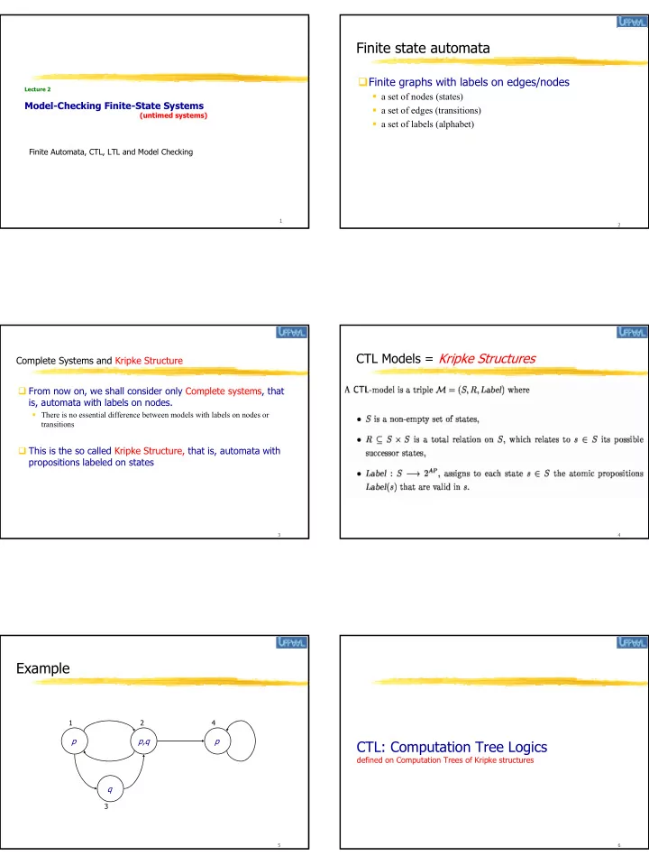
Example

p p q p,q

1 2 3 4

6

CTL: Computation Tree Logics

defined on Computation Trees of Kripke structures

7

Computation Tree Logic, CTL

Clarke & Emerson 1980

Syntax

8

Path

p p p

s s1 s2 s3...

The set of path starting in s

9

Formal Semantics

( )

10

CTL, Derived Operators

. . . . . . . . . . . . p p p AF p . . . . . . . . . . . . p EF p

possible inevitable E<> p in UPPAAL ! A<> p in UPPAAL

11

CTL, Derived Operators

p p p . . . . . . . . . . . . AG p p p p p p p . . . . . . . . . . . . EG p p

always potentially always A[] p in UPPAAL E[] p in UPPAAL

12

There are too many operators! But

We need to remember only the following:

X

(neXt time)

E F

(Future, some time)

A G

(Global)

U

(Until)

The most useful are EF, AG, EG and AF:

13

Theorem

All operators are derivable from

• EX f
• EG f
• E[ f U g ]

and boolean connectives All operators are derivable from

• EX f
• EG f
• E[ f U g ]

and boolean connectives

[ ] ( ) [ ]

g g f g g f ¬ ¬ ∧ ¬ ∧ ¬ ¬ ¬ ≡ EG U E U A

14

Example

p p q p,q

1 2 3 4

15

Example

p p q p,q

EX p

1 2 3 4

16

Example

p p q p,q

EX p

1 2 3 4

17

Example

p p q p,q

AX p

1 2 3 4

18

Example

p p q p,q

AX p

1 2 3 4

Note: state 1 doesn’t satisfy AX p

19

Example

p p q p,q

EG p

1 2 3 4

20

Example

p p q p,q

EG p

1 2 3 4

21

Example

p p q p,q

AG p

1 2 3 4

22

Example

p p q p,q

AG p

1 2 3 4

23

Example

p p q p,q

A[ p U q ]

1 2 3 4

24

Example

p p q p,q

A[ p U q ]

1 2 3 4

25

Properties of MUTEX example ?

I1 I2 t=0 T1 I2 t=0 T1 T2 t=0 I1 T2 t=0 I1 C2 t=0 T1 C2 t=0 C1 I2 t=1 T1 T2 t=1 C1 T2 t=1 T1 I2 t=1 I1 T2 t=1 I1 I2 t=1

[ ] [ ] ( ) [ ] [ ]

C U C A C U C A C AG C EG AF(C T AG[ C (C AG

2 1 1 1 1 1 1 1 2 1

¬ ∧ ¬ ⇒ ¬ ⇒ ∧ ¬ )] )

HOW to DECIDE IN GENERAL

26

CTL Model Checking Algorithms

27

Labeling Methods [Clarke et al 81]

Check all sub-formulas of F For each sub-formula f of F, label all nodes where f is true Check the composed formulas

28 29

Algorithm ideas for checking E(f U g)

Mark all nodes where f is true and all nodes where g is true Start from all nodes where g is true and Perform backwards reachability analysis Each step backwards, store all nodes in Q where f is true Repeat the above step, until it converges Q contains all nodes satisfying E(f U g)

Q Q + f Q=g

30

31

Algorithm ideas for checking A(f U g)

Similar to the case for A(f U g)

But each step backwards, store all nodes in Q where (f or g) is true, and the stored nodes do not lead to a node where (f or g) is false Repeat the above step, until it converges Q contains all nodes satisfying A(f U g)

Q Q+ f Not (f) Q=g

32

)) ( } ' ) ' , '.( | ({ φ Sat Q s R s s s s ∩ ∈ ⇒ ∈ ∀

33

Fixpoint Characterizations

p p p EF EX EF ∨ ≡

• r let A be the set of states satisfying EF p then

A EX A ∨ ≡ p

in fact A is the smallest one of sets satisfying the equations (the least fixpoint)

34

Fixed points of monotonic functions

Let τ be a function S → S Say τ is monotonic when Fixed point of τ is y such that If τ monotonic, then it has

least fixed point µy. τ(y) greatest fixed point νy. τ(y)

) ( ) ( implies y x y x τ τ ⊆ ⊆

y y = ) ( τ

35

Iteratively computing fixed points

Suppose S is finite

The least fixed point µy. τ(y) is the limit of The greatest fixed point νy. τ(y) is the limit of Λ ⊆ ⊆ ⊆ (false)) ( (false) false τ τ τ Λ ⊇ ⊇ ⊇ (true)) ( (true) true τ τ τ

Note, since S is finite, convergence is finite

36

Example: EF p

EF p is characterized by Thus, it is the limit of the increasing series...

) ( . y EX p y p EF ∨ = µ

p p ∨ EX p p ∨ EX(p ∨ EX p) . . .

37

Example: EG p

EG p is characterized by Thus, it is the limit of the decreasing series...

) ( . y EX p y p EG ∧ = ν

p ∧ EX p p p ∧ EX(p ∧ EX p) ...

38

Example, continued

p q p,q EF q p 1 2 3 4

} 3 , 2 , 1 { } 3 , 2 , 1 { } 3 , 2 {

3 2 1

= = = = A A A Ø A

) ( . y EX q y q EF ∨ = µ

39

Remaining operators

)) ( ( . ) ( )) ( ( . ) ( ) ( . ) ( . y AX p q y q U p A y EX p q y q U p E y AX p y p AG y AX p y p AF ∧ ∨ = ∧ ∨ = ∧ = ∨ = µ µ ν µ

40

Complexity

However Ssys may be EXPONENTIAL in number of parallel components!

• FIXPOINT COMPUTATIONS may be carried
• ut using

ROBDD’s (Reduced Ordered Binary Decision Diagrams) Bryant, 86 However Ssys may be EXPONENTIAL in number of parallel components!

• FIXPOINT COMPUTATIONS may be carried
• ut using

ROBDD’s (Reduced Ordered Binary Decision Diagrams) Bryant, 86

41

Something more about Finite State Automata and Temporal Logics

(Continuation of Lecture 2)

42

Branching time semantics

Computation tree of an automaton is the unfolding

• f the automaton

43

Example (Branching Time)

a a b a a a a a a b b b

44

Linear Time Semantics

Sequences of transitions (or states)

set of possible excecutions of a system

Suite best for closed systems

45

Example (Linear Time)

a a b a b a b a a b a a

46

Equivalences and Preorders

A equivalent to B if the tree of A is identical to the tree of B (Too strong!) A is simulated by B if every transition of A is simulated by a transition of B (simulation [Milner78]) A and B are bisimular if there is a symmetrical simulation between A’s and B’s states (bisimulation [Milner80]) A and B are testing equivalent if they can pass the same set

• f tests (may and must testing [Nicola and Hennessy 84])

A and B trace-equivalent if they provide the same set of sequences of transitions (trace equivalence [Hoare76])

47

LTL: Linear Time Logics

defined on infinite traces of Kripke structures with accepting conditions

48

Models: Infinite Sequences (ω-language accepted by automata) Automata with accepting conditions

Buchi, Muller automata

Infininte accepted sequences of transitions as semantics of automata

49

LTL: Syntax

P not F F1 and F2 O F (next time) F1 U F2 (Until)

50

LTL: semantics

assume an automaton M

a sequence of M: t=s(0)s(1)s(2)...s(i) ... ... The set of sequences of M is Comp(M)

s(i) sat p if p is a label of s(i)

s(i) sat not F if not (s(i) sat F) s(i) sat F1 and F2 if s(i) sat F1 and s(i) sat F2 s(i) sat O F if s(i+1) sat F s(i) sat F1 U F2 if s(k) sat F2 for some k=>i and s(j) sat F1 for all j such that i<=j<k

51

LTL: semantics (contn.)

assume an automaton M

a sequence of M: t=s(0)s(1)s(2)...s(i) ... ... The set of sequences of M is Comp(M)

t sat F iff s(0) sat F M sat F iff t sat F for all sequences t of Comp(M)

52

Derived Operators

<>F denotes (true U F) [ ]F denotes not (<> not F) F1 W F2 denotes (F1 U F2) or [ ]F1 (weak Until-operator)

53

Model Checking LTL [Wolper et al 1986]

Given an automata M and a formula F, to check M sat F

Construct the formula automaton: A(¬ F) Construct the product automaton M || A(¬ F) (on-the-fly)

If M || A(¬ F) is empty then M sat F otherwise NO Time-Complexity = |M|*2O(|F|)

The same idea can be used for CTL model checking using Tree-automata

54

Comparing CTL and LTL

<> P (LTL) similar AF p (CTL) [] p (LTL) similar AG p (CTL) However,

LTL cannot express possibilities properties: EF P CTL cannot express <>[] p CTL* = LTL + CTL

55

Comparing CTL and LTL (contn.)

¬P Satisfies <>[] p but it does not satisfy AF AG p P P

56

Why?

p p p ¬p ¬p ¬p p p p No subtree where p is true everywhere

57

END (Finite State Untimed Systems)