BIL 717 Image Processing Linear Filtering Review Feb. 15, 2016 - - PowerPoint PPT Presentation

BIL 717 Image Processing

• Feb. 15, 2016

Linear Filtering Edge Detection

Erkut Erdem

Hacettepe University Computer Vision Lab (HUCVL)

Today

• Linear Filtering

– Review – Gauss filter – Linear diffusion

• Edge Detection

– Review – Derivative filters – Laplacian of Gaussian – Canny edge detector

Today

• Linear Filtering

– Review – Gauss filter – Linear diffusion

• Edge Detection

– Review – Derivative filters – Laplacian of Gaussian – Canny edge detector

Filtering

• The name “filter” is borrowed from frequency domain

processing

• Accept or reject certain frequency components
• Fourier (1807):

Periodic functions could be represented as a weighted sum of sines and cosines

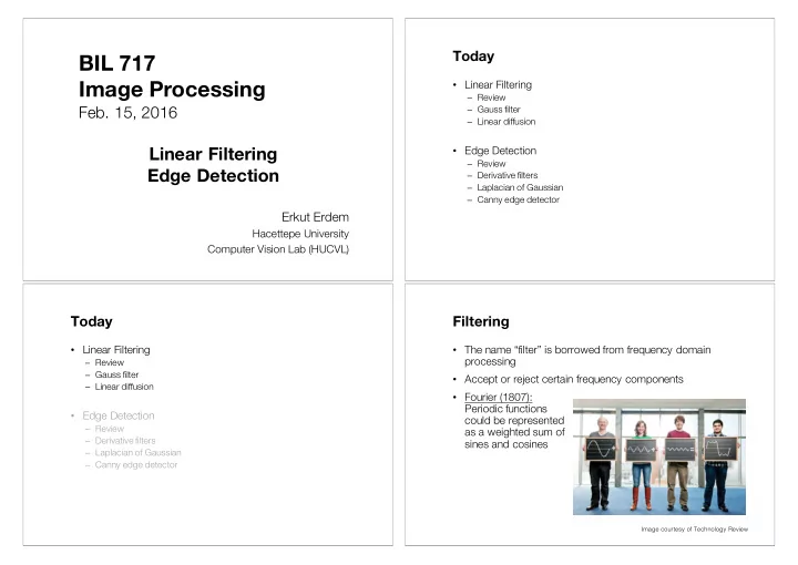
Image courtesy of Technology Review

Signals

• A signal is composed of low and high frequency

components

low frequency components: smooth / piecewise smooth high frequency components: oscillatory Neighboring pixels have similar brightness values Neighboring pixels have different brightness values You’re within a region You’re either at the edges or noise points

Signals – Examples Motivation: noise reduction

• Assume image is degraded with an additive model.
• Then,

Observation = True signal + noise Observed image = Actual image + noise

low-pass filters smooth the image

Common types of noise

– Salt and pepper noise: random occurrences of black and white pixels – Impulse noise: random occurrences of white pixels – Gaussian noise: variations in intensity drawn from a Gaussian normal distribution

Slide credit: S. Seitz

Gaussian noise

Slide credit: M. Hebert

>> noise = randn(size(im)).*sigma; >> output = im + noise;

What is the impact of the sigma?

Motivation: noise reduction

• Make multiple observations of the same static scene
• Take the average
• Even multiple images of the same static scene will not be

identical.

Adapted from: K. Grauman

Motivation: noise reduction

• Make multiple observations of the same static scene
• Take the average
• Even multiple images of the same static scene will not be

identical.

• What if we can’t make multiple observations?

What if there’s only one image?

Adapted from: K. Grauman

Image Filtering

• Idea: Use the information coming from the

neighboring pixels for processing

• Design a transformation function of the local

neighborhood at each pixel in the image

– Function specified by a “filter” or mask saying how to combine values from neighbors.

• Various uses of filtering:

– Enhance an image (denoise, resize, etc) – Extract information (texture, edges, etc) – Detect patterns (template matching)

Adapted from: K. Grauman

Filtering

• Processing done on a function

– can be executed in continuous form (e.g. analog circuit) – but can also be executed using sampled representation

• Simple example: smoothing by averaging

Slide credit: S. Marschner

Linear filtering

• Filtered value is the linear combination of neighboring

pixel values.

• Key properties

– linearity: filter(f + g) = filter(f) + filter(g) – shift invariance: behavior invariant to shifting the input

• delaying an audio signal
• sliding an image around
• Can be modeled mathematically by convolution

Adapted from: S. Marschner

First attempt at a solution

• Let’s replace each pixel with an average of all the values in

its neighborhood

• Assumptions:

– Expect pixels to be like their neighbors (spatial regularity in images) – Expect noise processes to be independent from pixel to pixel

Slide credit: S. Marschner, K. Grauman

First attempt at a solution

• Let’s replace each pixel with an average of all the values in

its neighborhood

• Moving average in 1D:

Slide credit: S. Marschner

Discrete convolution

• Simple averaging:

– every sample gets the same weight

• Convolution: same idea but with weighted average

– each sample gets its own weight (normally zero far away)

• This is all convolution is: it is a moving weighted average

Slide credit: S. Marschner

Filters

• Sequence of weights a[j] is called a filter
• Filter is nonzero over its region of support

– usually centered on zero: support radius r

• Filter is normalized so that it sums to 1.0

– this makes for a weighted average, not just any

• ld weighted sum
• Most filters are symmetric about 0

– since for images we usually want to treat left and right the same

a box filter

Slide credit: S. Marschner

Convolution and filtering

• Can express sliding average as convolution with a box filter
• abox = […, 0, 1, 1, 1, 1, 1, 0, …]

Slide credit: S. Marschner

Example: box and step

Slide credit: S. Marschner

Convolution and filtering

• Convolution applies with any sequence of weights
• Example: bell curve (gaussian-like) […, 1, 4, 6, 4, 1, …]/16

Slide credit: S. Marschner

And in pseudocode…

Slide credit: S. Marschner

Key properties

• Linearity: filter(f1 + f2) = filter(f1) + filter(f2)
• Shift invariance: filter(shift(f)) = shift(filter(f))
• same behavior regardless of pixel location, i.e. the value of the output

depends on the pattern in the image neighborhood, not the position

• f the neighborhood.
• Theoretical result: any linear shift-invariant operator can be

represented as a convolution

Slide credit: S. Lazebnik

Properties in more detail

• Commutative: a * b = b * a

– Conceptually no difference between filter and signal

• Associative: a * (b * c) = (a * b) * c

– Often apply several filters one after another: (((a * b1) * b2) * b3) – This is equivalent to applying one filter: a * (b1 * b2 * b3)

• Distributes over addition: a * (b + c) = (a * b) + (a * c)
• Scalars factor out: ka * b = a * kb = k (a * b)
• Identity: unit impulse e = […, 0, 0, 1, 0, 0, …],

a * e = a

Slide credit: S. Lazebnik

Discrete filtering in 2D

• Same equation, one more index

– now the filter is a rectangle you slide around over a grid of numbers

• Usefulness of associativity

– often apply several filters one after another: (((a * b1) * b2) * b3) – this is equivalent to applying one filter: a * (b1 * b2 * b3)

Slide credit: S. Marschner

And in pseudocode…

Slide credit: S. Marschner

Moving Average In 2D

90 90 90 90 90 90 90 90 90 90 90 90 90 90 90 90 90 90 90 90 90 90 90 90 90 90 90 90 90 90 90 90 90 90 90 90 90 90 90 90 90 90 90 90 90 90 90 90 90 90

Slide credit: S. Seitz

Moving Average In 2D

90 90 90 90 90 90 90 90 90 90 90 90 90 90 90 90 90 90 90 90 90 90 90 90 90 10 90 90 90 90 90 90 90 90 90 90 90 90 90 90 90 90 90 90 90 90 90 90 90 90 90

Slide credit: S. Seitz

Moving Average In 2D

90 90 90 90 90 90 90 90 90 90 90 90 90 90 90 90 90 90 90 90 90 90 90 90 90 10 20 30 30 30 20 10 20 40 60 60 60 40 20 30 60 90 90 90 60 30 30 50 80 80 90 60 30 30 50 80 80 90 60 30 20 30 50 50 60 40 20 10 20 30 30 30 30 20 10 10 10 10

Slide credit: S. Seitz

Averaging filter

• What values belong in the kernel H for the moving

average example?

10 20 30 30 90 90 90 90 90 90 90 90 90 90 90 90 90 90 90 90 90 90 90 90 90 90 90 90 90

1 1 1 1 1 1 1 1 1 “box filter”

?

Slide credit: K. Grauman

Smoothing by averaging

depicts box filter: white = high value, black = low value

• riginal

filtered

What if the filter size was 5 x 5 instead of 3 x 3?

Slide credit: K. Grauman

Boundary issues

• What is the size of the output?
• MATLAB: output size / “shape” options

– shape = ‘full’: output size is sum of sizes of f and g – shape = ‘same’: output size is same as f – shape = ‘valid’: output size is difference of sizes of f and g

f g g g g f g g g g f g g g g full same valid

Slide credit: S. Lazebnik

Boundary issues

• What about near the edge?

– the filter window falls off the edge of the image – need to extrapolate – methods:

• clip filter (black)
• wrap around
• copy edge
• reflect across edge

Slide credit: S. Marschner

Boundary issues

• What about near the edge?

– the filter window falls off the edge of the image – need to extrapolate – methods (MATLAB):

• clip filter (black):

imfilter(f, g, 0)

• wrap around:

imfilter(f, g, ‘circular’)

• copy edge:

imfilter(f, g, ‘replicate’)

• reflect across edge:

imfilter(f, g, ‘symmetric’)

Slide credit: S. Marschner

Gaussian filter

90 90 90 90 90 90 90 90 90 90 90 90 90 90 90 90 90 90 90 90 90 90 90 90 90 1 2 1 2 4 2 1 2 1

• What if we want nearest neighboring pixels to have the

most influence on the output?

• Removes high-frequency components from the image

(“low-pass filter”).

This kernel is an approximation of a 2d Gaussian function:

Slide credit: S. Seitz

Smoothing with a Gaussian

Slide credit: K. Grauman

Gaussian filters

• What parameters matter here?
• Size of kernel or mask

– Note, Gaussian function has infinite support, but discrete filters use finite kernels

σ = 5 with 10 x 10 kernel σ = 5 with 30 x 30 kernel

Slide credit: K. Grauman

Gaussian filters

• What parameters matter here?
• Variance of Gaussian: determines extent of

smoothing

σ = 2 with 30 x 30 kernel σ = 5 with 30 x 30 kernel

Slide credit: K. Grauman

Matlab

>> hsize = 10; >> sigma = 5; >> h = fspecial(‘gaussian’ hsize, sigma); >> mesh(h); >> imagesc(h); >> outim = imfilter(im, h); % correlation >> imshow(outim);

• utim

Slide credit: K. Grauman

Smoothing with a Gaussian

for sigma=1:3:10 h = fspecial('gaussian‘, fsize, sigma);

• ut = imfilter(im, h);

imshow(out); pause; end

…

Parameter σ is the “scale” / “width” / “spread” of the Gaussian kernel, and controls the amount of smoothing.

Slide credit: K. Grauman

Properties of smoothing filters

• Smoothing

– Values positive – Sum to 1 à constant regions same as input – Amount of smoothing proportional to mask size – Remove “high-frequency” components; “low-pass” filter

Slide credit: K. Grauman

Linear Diffusion

• Let f (x) denote a grayscale (noisy) input image and u(x, t) be

initialized with u(x,0) = u0(x) = f(x).

• The linear diffusion process can be defined by the equation:

where · denotes the divergence operator. Thus, ) ∂u ∂t = ∇ · (∇u) = ∇2u ) ∂u ∂t = ∂2u ∂x2 + ∂2u ∂y2

Linear Diffusion (cont’d.)

• Diffusion process as an evolution process.
• Artificial time variable t denotes the diffusion time
• Input image is smoothed at a constant rate in all

directions.

– u0(x): initial image, – u(x, t): the evolving images under the governed equation representing the successively smoothed versions of the initial input image f (x).

• Diffusion process creates a scale space representation
• f the given image f , with t > 0 being the scale.

Linear Diffusion (cont’d.)

) ∂u ∂t = ∇ · (∇u) = ∇2u

red: active areas blue: inactive area influence of the central pixel

• n the other pixels

(red: high, blue: low)

gray-level image

Credit: S. Paris

Linear Diffusion (cont’d.)

• As we move to coarser scales,

– Evolving images become more and more simplified – Diffusion process removes the image structures at finer scales.

T = 0 T = 1.25 T = 2.5 T = 5 T = 10 T = 20

Linear Diffusion (cont’d.)

• As we move to coarser scales,

– Evolving images become more and more simplified – Diffusion process removes the image structures at finer scales.

T = 0 T = 5 T = 10 T = 20 T = 40 T = 80

Linear Diffusion and Gaussian Filtering

• The solution of the linear diffusion can be explicitly estimated

as: with

• Solution of the linear diffusion equation is equivalent to a

proper convolution of the input image with the Gaussian kernel Gσ(x) with standard deviation

• The higher the value of T, the higher the value of σ, and the

more smooth the image becomes.

) u(x, T) =

• G√

2T ∗ f

• (x)

Gσ(x) = 1 2πσ2 exp

• −|x|2

2σ2

• tion of the in

σ = √ 2T [2 respondenc

Numerical Implementation

• Solving the linear diffusion equation requires discretization in

both spatial and time coordinates.

• Central differences for the spatial derivatives:

where ui,j denotes the gray value or the brightness of the evolving image at pixel location (i, j).

• We take hx = hy = 1 for a regular grid.

) d2ui,j dx2 ≈ ui+hx,j − 2ui,j + ui−hx,j h2

x

d2ui,j dy2

≈

ui,j+hy − 2ui,j + ui,j−hy h2

y

Numerical Implementation (cont’d.)

• Original model:
• Space discrete version:
• Space-time discrete version:

) ∂u ∂t = ∂2u ∂x2 + ∂2u ∂y2 ) dui,j dt

= ui+1,j + ui−1,j + ui,j+1 + ui,j−1 − 4ui,j

) uk+1

i,j

− uk

i,j

∆t = uk

i+1,j + uk i−1,j + uk i,j+1 + uk i,j−1 − 4uk i,j homogeneous Neumann boundary condition along the image boundary ∆t ≤ 0.25 is required for numerical stability

Variational Regularization

• Variational regularization models formulate smoothing

process as a functional minimization via which a noise-free approximation of a given image is to be estimated.

• With an additive model, f(x) = u(x) + n(x)

– f(x): original image – u(x): smoothed image – n(x): noise component

• An example: Tikhonov energy functional

) E(u) =

• Ω
• (u − f )2 + α|∇u|2

dx

Tikhonov energy functional

• Ω R2 is connected, bounded, open subset representing

the image domain,

• f is an image defined on Ω,
• u is the smooth approximation of f ,
• α > 0 is the scale parameter.

) E(u) =

• Ω
• (u − f )2 + α|∇u|2

dx

data fidelity term regularization term

Variational Regularization and Diffusion Equations

• A strong relation between variational regularization methods

and diffusion equations.

• The minimizing function u of the Tikhonov energy functional

formally satisfies the Euler-Lagrange equation: with the Neumann boundary condition

• can be rewritten as:

) (u − f ) − α∇2u = 0

ion ∂u

∂n

• ∂Ω = 0.

0) u − u0 α = ∇2u with u0 = f,

implicit time discretization of the linear diffusion equation with a single time step (T = α)

Today

• Linear Filtering

– Review – Gauss filter – Linear diffusion

• Edge Detection

– Review – Derivative filters – Laplacian of Gaussian – Canny edge detector

Signals and Images

• A signal is composed of low and high frequency

components

low frequency components: smooth / piecewise smooth high frequency components: oscillatory Neighboring pixels have similar brightness values Neighboring pixels have different brightness values You’re within a region You’re either at the edges or noise points

Edge detection

• Goal: Identify sudden changes

(discontinuities) in an image

– Intuitively, most semantic and shape information from the image can be encoded in the edges – More compact than pixels

• Ideal: artist’s line drawing (but

artist is also using object-level knowledge)

Slide credit: D. Lowe

Why do we care about edges?

• Extract information, recognize
• bjects
• Recover geometry and viewpoint

Vanishing point Vanishing line Vanishing point Vertical vanishing point (at infinity)

Source: J. Hays

Closeup of edges

Slide credit: D. Hoiem

What causes an edge?

Depth discontinuity:

• bject boundary

Change in surface

• rientation: shape

Cast shadows Reflectance change: appearance information, texture

Slide credit: K. Grauman

Characterizing edges

• An edge is a place of rapid change in the image

intensity function

image intensity function (along horizontal scanline) first derivative edges correspond to extrema of derivative

Slide credit: K. Grauman

Derivatives with convolution

For 2D function f(x,y), the partial derivative is: For discrete data, we can approximate using finite differences: To implement above as convolution, what would be the associated filter?

ε ε

ε

) , ( ) , ( lim ) , ( y x f y x f x y x f − + = ∂ ∂

→

1 ) , ( ) , 1 ( ) , ( y x f y x f x y x f − + ≈ ∂ ∂

Slide credit: K. Grauman

Partial derivatives of an image

• 1

1

• 1 1

x y x f ∂ ∂ ) , ( y y x f ∂ ∂ ) , (

Which shows changes with respect to x?

Slide credit: K. Grauman

Assorted finite difference filters

>> My = fspecial(‘sobel’); >> outim = imfilter(double(im), My); >> imagesc(outim); >> colormap gray;

Slide credit: K. Grauman

The gradient points in the direction of most rapid increase in intensity

Image gradient

• The gradient of an image:
• The gradient direction is given by

Slide credit: S. Seitz

The edge strength is given by the gradient magnitude

• How does this direction relate to the direction of the edge?

Original Image

Slide credit: K. Grauman

Gradient magnitude image

Slide credit: K. Grauman

Thresholding gradient with a lower threshold

Slide credit: K. Grauman

Thresholding gradient with a higher threshold

Slide credit: K. Grauman

Intensity profile

Slide credit: D. Hoiem

With a little Gaussian noise

Gradient

Slide credit: D. Hoiem

Effects of noise

• Consider a single row or column of the image

– Plotting intensity as a function of position gives a signal

Where is the edge?

Slide credit: S. Seitz

Effects of noise

• Difference filters respond strongly to noise

– Image noise results in pixels that look very different from their neighbors – Generally, the larger the noise the stronger the response

• What can we do about it?

Slide credit: D. Forsyth

Solution: smooth first

• To find edges, look for peaks in

) ( g f dx d ∗ f g f * g

) ( g f dx d ∗

Slide credit: S. Seitz

Smoothing with a Gaussian

Recall: parameter σ is the scale / width / spread of the Gaussian kernel, and controls the amount of smoothing.

…

Slide credit: K. Grauman

Effect of σ on derivatives

The apparent structures differ depending on Gaussians scale parameter. Larger values: larger scale edges detected Smaller values: finer features detected

σ = 1 pixel σ = 3 pixels

Slide credit: K. Grauman

So, what scale to choose?

It depends what we’re looking for.

Slide credit: K. Grauman

Smoothing and Edge Detection

• While eliminating noise via smoothing, we also lose some of

the (important) image details.

– Fine details – Image edges – etc.

• What can we do to preserve such details?

– Use edge information during denoising! – This requires a definition for image edges.

• Edge preserving image smoothing (Next week’s topic!)

Chicken-and-egg dilemma!

• Differentiation is convolution, and convolution is associative:
• This saves us one operation:

g dx d f g f dx d ∗ = ∗ ) (

Derivative theorem of convolution

g dx d f ∗

f

g dx d

Slide credit: S. Seitz

Derivative of Gaussian filter

x-direction y-direction

Slide credit: S. Lazebnik

* [1 -1] =

Derivative of Gaussian filter

• Which one finds horizontal/vertical edges?

x-direction y-direction

Slide credit: S. Lazebnik

Smoothing vs. derivative filters

• Smoothing filters

– Gaussian: remove “high-frequency” components; “low-pass” filter – Can the values of a smoothing filter be negative? – What should the values sum to?

• One: constant regions are not affected by the filter
• Derivative filters

– Derivatives of Gaussian – Can the values of a derivative filter be negative? – What should the values sum to?

• Zero: no response in constant regions

– High absolute value at points of high contrast

Slide credit: S. Lazebnik

Laplacian of Gaussian

Consider

Laplacian of Gaussian

• perator

Where is the edge? Zero-crossings of bottom graph

Slide credit: K. Grauman

2D edge detection filters

• The Laplacian operator:

Laplacian of Gaussian Gaussian derivative of Gaussian

Slide credit: K. Grauman

Laplacian of Gaussian

• riginal image

Source: D. Marr and E. Hildreth (1980)

Laplacian of Gaussian

convolution with

Source: D. Marr and E. Hildreth (1980)

Laplacian of Gaussian

convolution with

(pos. values – white, neg. values – black)

Source: D. Marr and E. Hildreth (1980)

Laplacian of Gaussian

zero-crossings

Source: D. Marr and E. Hildreth (1980)

Designing an edge detector

• Criteria for a good edge detector:

– Good detection: the optimal detector should find all real edges, ignoring noise or other artifacts – Good localization

• the edges detected must be as close as possible to the true edges
• the detector must return one point only for each true edge point
• Cues of edge detection

– Differences in color, intensity, or texture across the boundary – Continuity and closure – High-level knowledge

Slide credit: L. Fei-Fei

The Canny edge detector

• riginal image (Lena)

Slide credit: K. Grauman

The Canny edge detector

norm of the gradient

thresholding

Slide credit: K. Grauman

The Canny edge detector

thresholding

How to turn these thick regions of the gradient into curves?

Slide credit: K. Grauman

Non-maximum suppression

Check if pixel is local maximum along gradient direction, select single max across width of the edge

– requires checking interpolated pixels p and r

Slide credit: K. Grauman

The Canny Edge Detector

thinning (non-maximum suppression) Problem: pixels along this edge didn’t survive the thresholding

Slide credit: K. Grauman

Hysteresis thresholding

• Threshold at low/high levels to get weak/strong edge pixels
• Do connected components, starting from strong edge pixels

Slide credit: J. Hays

Hysteresis thresholding

• Check that maximum value of gradient value is

sufficiently large

– drop-outs? use hysteresis

• use a high threshold to start edge curves and a low threshold to

continue them.

Slide credit: S. Seitz

Hysteresis thresholding

• riginal image

high threshold (strong edges) low threshold (weak edges) hysteresis threshold

Slide credit: L. Fei-Fei

• riginal image

high threshold (strong edges) low threshold (weak edges) hysteresis threshold

Slide credit: L. Fei-Fei

Hysteresis thresholding

Recap: Canny edge detector

1. Filter image with derivative of Gaussian 2. Find magnitude and orientation of gradient 3. Non-maximum suppression: – Thin wide “ridges” down to single pixel width 4. Linking and thresholding (hysteresis): – Define two thresholds: low and high – Use the high threshold to start edge curves and the low threshold to continue them

• MATLAB: edge(image, ‘canny’);

Slide credit: D. Lowe, L. Fei-Fei

Effect of σ (Gaussian kernel spread/size)

Canny with Canny with

• riginal

The choice of σ depends on desired behavior

• large σ detects large scale edges
• small σ detects fine features

Slide credit: S. Seitz

Background Texture Shadows

Low-level edges vs. perceived contours

Slide credit: K. Grauman

Edge detection is just the beginning…

• Berkeley segmentation database:

http://www.eecs.berkeley.edu/Research/Projects/CS/vision/grouping/segbench/

image human segmentation gradient magnitude

Source: S. Lazebnik

[D. Martin et al. PAMI 2004]

Human-marked segment boundaries

Learn from humans which combination of features is most indicative

• f a “good”

contour?

Slide credit: K. Grauman