[PPT] - BIL 717 Image Processing Active Contours Variational PowerPoint Presentation

SLIDE 1

BIL 717 Image Processing

Mar. 7, 2016

Active Contours/Snakes Variational Segmentation Models

Erkut Erdem

Hacettepe University Computer Vision Lab (HUCVL)

Acknowledgement: The slides on active contours are adapted from the slides prepared by K. Grauman of University

f Texas at Austin

Today

Active Contours
Variational Segmentation Models

Today

Active Contours
Variational Segmentation Models

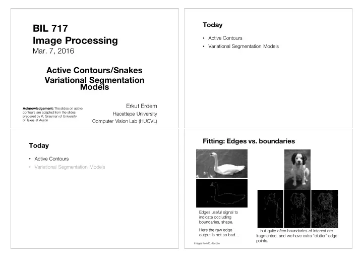
Fitting: Edges vs. boundaries

Edges useful signal to indicate occluding boundaries, shape. Here the raw edge

utput is not so bad…

…but quite often boundaries of interest are fragmented, and we have extra “clutter” edge points.

Images from D. Jacobs

SLIDE 2

Given a model of interest, we can overcome some of the missing and noisy edges using fitting techniques. With voting methods like the Hough transform, detected points vote on possible model parameters.

Fitting: Edges vs. boundaries Deformable contours

Given: initial contour (model) near desired object

a.k.a. active contours, snakes

Figure credit: Yuri Boykov

Goal: evolve the contour to fit exact object boundary

[Snakes: Active contour models, Kass, Witkin, & T erzopoulos, ICCV1987]

Main idea: elastic band is iteratively adjusted so as to

be near image positions with

high gradients, and

satisfy shape “preferences” or

contour priors

Deformable contours: intuition

Image from http://www.healthline.com/blogs/exercise_fitness/up loaded_images/H and Band 2-795868.JPG

Deformable contours vs. Hough

initial intermediate final

Like generalized Hough transform, useful for shape fitting; but Hough Rigid model shape Single voting pass can detect multiple instances Deformable contours Prior on shape types, but shape iteratively adjusted (deforms) Requires initialization nearby One optimization “pass” to fit a single contour

SLIDE 3

Why do we want to fit deformable shapes?

Some objects have similar basic form but

some variety in the contour shape.

Figure credit: Julien Jomier

Why do we want to fit deformable shapes?

Non-rigid, deformable objects can change their shape
ver time.

Aspects we need to consider

Representation of the contours
Defining the energy functions

– External – Internal

Minimizing the energy function

Representation

We’ll consider a discrete representation of the contour,

consisting of a list of 2d point positions (“vertices”).

), , (

i i i

y x = ν 1 , , 1 , − = n i !

for

At each iteration, we’ll have the option

to move each vertex to another nearby location (“state”).

) , (

0 y

x ) , (

19 19 y

x

SLIDE 4

Fitting deformable contours

initial intermediate final

How should we adjust the current contour to form the new contour at each iteration?

Define a cost function (“energy” function) that says how good a

candidate configuration is.

Seek next configuration that minimizes that cost function.

Energy function

The total energy (cost) of the current snake is defined as: external internal total

E E E + =

A good fit between the current deformable contour and the target shape in the image will yield a low value for this cost function. Internal energy: encourage prior shape preferences: e.g., smoothness, elasticity, particular known shape. External energy (“image” energy): encourage contour to fit on places where image structures exist, e.g., edges.

External energy: intuition

Measure how well the curve matches the image data
“Attract” the curve toward different image features

– Edges, lines, texture gradient, etc.

External image energy

Magnitude of gradient

(Magnitude of gradient)

( )

2 2

) ( ) ( I G I G

y x

+ −

2 2

) ( ) ( I G I G

y x

+

How do edges affect “snap” of rubber band? Think of external energy from image as gravitational pull towards areas of high contrast

SLIDE 5

Gradient images and
External energy at a point on the curve is:
External energy for the whole curve:

) , ( y x Gx ) , ( y x Gy

) | ) ( | | ) ( | ( ) (

2 2

ν ν ν

y x external

G G E + − =

External image energy

2 1 2

| ) , ( | | ) , ( |

i i y n i i i x external

y x G y x G E

∑

− =

+ − =

Internal energy: intuition

What are the underlying boundaries in this fragmented edge image? And in this one? A priori, we want to favor smooth shapes, contours with low curvature, contours similar to a known shape, etc. to balance what is actually observed (i.e., in the gradient image).

Internal energy: intuition Internal energy

For a continuous curve, a common internal energy term is the “bending energy”. At some point v(s) on the curve, this is:

Tension, Elasticity Stiffness, Curvature

s d d ds d

s Einternal 2 2 )) ( (

2 2

ν ν

β α ν + =

SLIDE 6

For our discrete representation,
Internal energy for the whole curve:

1 ) , ( − = = n i y x

i i i

! ν

i 1 i

v ds d ν ν − ≈

+ 1 1 1 1 2 2

2 ) ( ) (

− + − +

+ − = − − − ≈

i i i i i i i

ds d ν ν ν ν ν ν ν ν

∑

− = − + +

+ − + − =

1 2 1 1 2 1

2

n i i i i i i internal

E ν ν ν β ν ν α

…

Internal energy

Note these are derivatives relative to position---not spatial image gradients. Why do these reflect tension and curvature?

Example: compare curvature

(1,1) (1,1) (2,2) (3,1) (3,1) (2,5)

2 1 1

2 ) (

− +

+ − =

i i i i curvature v

E ν ν ν

2 1 1 2 1 1

) 2 ( ) 2 (

− + − +

+ − + + − =

i i i i i i

y y y x x x

Penalizing elasticity

Current elastic energy definition uses a discrete estimate
f the derivative:

What is the possible problem with this definition?

2 1 1 2 1

) ( ) (

i i n i i i

y y x x − + − ⋅ =

+ − = +

∑

α

∑

− = + −

=

1 2 1 n i i i elastic

E ν ν α

Penalizing elasticity

Current elastic energy definition uses a discrete estimate
f the derivative:

∑

− = + −

=

1 2 1 n i i i elastic

E ν ν α

( )

2 1 2 1 2 1

) ( ) (

∑

− = + +

− − + − ⋅ =

n i i i i i

d y y x x α

where d is the average distance between pairs

f points – updated at each iteration.

Instead:

SLIDE 7

Dealing with missing data

The preferences for low-curvature, smoothness help deal

with missing data:

[Figure from Kass et al. 1987]

Illusory contours found!

Extending the internal energy: capture shape prior

If object is some smooth variation on a

known shape, we can use a term that will penalize deviation from that shape:

where are the points of the known shape.

∑

− =

− ⋅ = +

1 2

) ˆ (

n i i i internal

E ν ν α

} ˆ {

i

ν

Fig from Y. Boykov

Total energy: function of the weights

external internal total

E E E γ + = ( )

∑

− = − + +

+ − + − − =

1 2 1 1 2 1

2

n i i i i i i internal

d E ν ν ν β ν ν α

2 1 2

| ) , ( | | ) , ( |

i i y n i i i x external

y x G y x G E

∑

− =

+ − =

α

large α small α medium α

e.g., weight controls the penalty for internal elasticity

Fig from Y. Boykov

Total energy: function of the weights

SLIDE 8

Recap: deformable contour

A simple elastic snake is defined by:

– A set of n points, – An internal energy term (tension, bending, plus optional shape prior) – An external energy term (gradient-based)

To use to segment an object:

– Initialize in the vicinity of the object – Modify the points to minimize the total energy

Energy minimization

Several algorithms have been proposed to fit

deformable contours:

– Greedy search – Dynamic programming (for 2d snakes) – etc.

Energy minimization: greedy

For each point, search window around it

and move to where energy function is minimal

– Typical window size, e.g., 5 x 5 pixels

Stop when predefined number of points

have not changed in last iteration, or after max number of iterations

Note:

– Convergence not guaranteed – Need decent initialization

1

v

2

v

3

v

4

v

6

v

5

v

With this form of the energy function, we can minimize using dynamic programming, with the Viterbi algorithm. Iterate until optimal position for each point is the center of the box, i.e., the snake is optimal in the local search space constrained by boxes.

[Amini, Weymouth, Jain, 1990] Fig from Y. Boykov

Energy minimization: dynamic programming

SLIDE 9

Energy minimization: dynamic programming

∑

− = +

=

1 1 1 1

) , ( ) , , (

n i i i i n total

E E ν ν ν ν !

Possible because snake energy can be rewritten as a sum of

pair-wise interaction potentials:

Or sum of triple-interaction potentials.

∑

− = + −

=

1 1 1 1 1

) , , ( ) , , (

n i i i i i n total

E E ν ν ν ν ν !

Snake energy: pair-wise interactions

2 1 1 2 1 1

| ) , ( | | ) , ( | ) , , , , , (

i i y n i i i x n n total

y x G y x G y y x x E

∑

− =

+ − = ! !

2 1 1 1 2 1

) ( ) (

i i n i i i

y y x x − + − ⋅ +

+ − = +

∑

α

∑

− =

1 1 2 1

|| ) ( || ) , , (

n i i n total

G E ν ν ν !

∑

− = + −

⋅ +

1 1 2 1

|| ||

n i i i

ν ν α ) , ( ... ) , ( ) , ( ) , , (

1 1 3 2 2 2 1 1 1 n n n n total

v v E v v E v v E E

− −

+ + + = ν ν !

2 1 2 1

|| || || ) ( || ) , (

i i i i i i

G E ν ν α ν ν ν − + − =

+ +

where Re-writing the above with : ( )

i i i

y x v , =

Kristen Grauman

) , ( ... ) , ( ) , (

1 1 3 2 2 2 1 1 n n n

v v E v v E v v E

− −

+ + +

DP can be applied to optimize an open ended snake For a closed snake, a “loop” is introduced into the total energy.

1

ν

n

ν

) , ( ) , ( ... ) , ( ) , (

1 1 1 3 2 2 2 1 1

v v E v v E v v E v v E

n n n n n

+ + + +

− −

1

ν

n

ν

2

ν

1 − n

ν

3

ν

4

ν Work around: 1) Fix v1 and solve for rest . 2) Fix an intermediate node at its position

Energy minimization: dynamic programming

May over-smooth the boundary
Cannot follow topological changes of objects

Limitations

SLIDE 10

Limitations

External energy: snake does not really “see” object

boundaries in the image unless it gets very close to it.

image gradients are large only directly on the boundary

I ∇

Distance transform

External image can instead be taken from the distance

transform of the edge image.

riginal
gradient

distance transform edges

Value at (x,y) tells how far that position is from the nearest edge point (or other binary mage structure)

>> help bwdist

Deformable contours: pros and cons

Pros:

Useful to track and fit non-rigid shapes
Contour remains connected
Possible to fill in “subjective” contours
Flexibility in how energy function is defined, weighted.

Cons:

Must have decent initialization near true boundary, may

get stuck in local minimum

Parameters of energy function must be set well based on

prior information

Summary

Deformable shapes and active contours are useful for

– Segmentation: fit or “snap” to boundary in image – Tracking: previous frame’s estimate serves to initialize the next

Fitting active contours:

– Define terms to encourage certain shapes, smoothness, low curvature, push/pulls, … – Use weights to control relative influence of each component cost – Can optimize 2d snakes with Viterbi algorithm.

Image structure (esp. gradients) can act as attraction force

for interactive segmentation methods.

SLIDE 11

Today

Active Contours
Variational Segmentation Models

Review – Nonlinear Diffusion

use nonlinear PDEs to create a scale space

representation

– consists of gradually simplified images – some image features such as edges are maintained or even enhanced.

Perona-Malik Type Nonlinear Diffusion (1990)
Total Variation (TV) Regularization (1992)
Weickert’s Edge Enhancing Diffusion (1994)

Review - Perona-Malik Type Nonlinear Diffusion

Perona-Malik equation is:

with homogeneous Neumann boundary conditions and the initial condition u0(x) = f (x), f denoting the input image.

Constant diffusion coefficient of linear equation is replaced

with a smooth non-increasing diffusivity function g satisfying – g(0) = 1, – g(s) ≥ 0, – lims→∞ g(s) = 0

The diffusivities become variable in both space and time.

∂u ∂t = r · (g(|ru|)ru)

Review - Perona-Malik Type Nonlinear Diffusion

Smoothing process diminishes noise while retaining or

enhancing edges

T = 0 T = 50 T = 100 T = 200 T = 400 T = 800

time (λ = 1, σ = 1).

SLIDE 12

Review - Total Variation (TV) Regularization

Rudin et al. (1992) formulated image restoration as

minimization of the total variation (TV) of a given image under certain assumptions on the noise.

Total Variation (TV) regularization model is generally defined

as:

– Ω R2 is connected, bounded, open subset representing the image domain, – f is an image defined on Ω, – u is the smooth approximation of f , – α > 0 is a scalar.

ETV(u) =

Z

Ω

✓1 2(u f )2 + α|ru| ◆ dx

Review - Total Variation (TV) Regularization

Total Variation (TV) regularization model:
The gradient descent equation for Equation (10) is defined

by:

The value of α specifies the relative importance of the fidelity

term.

It can be interpreted as a scale parameter that determines

the level of smoothing. ETV(u) =

Z

Ω

✓1 2(u f )2 + α|ru| ◆ dx

(11) ∂u ∂t = r · ✓ ru |ru| ◆ 1 a(u f ); ∂u ∂n

∂Ω

= 0 .

Review - TV Restoration results

(b) α = 50, (c) α = 100, (d) α = 200.

The value of α specifies the relative importance of the fidelity

term and thus the level of smoothing.

Review - TV Regularization and TV Flow

TV regularization can be associated with a nonlinear diffusion

filter, the so-called TV flow

Ignoring the fidelity term in the TV regularization model

leads to the PDE: with and the diffusivity function

Notice that this diffusivity function has no additional contrast

parameter as compared with the Perona-Malik diffusivities.

∂u ∂t = r · (g(|ru|)ru)

with u0 = f and function g(|ru|) =

1 |ru|.

parameter as compared

SLIDE 13

Review - Sample TV Flow results

Corresponding smoothing process yields segmentation-like,

piecewise constant images.

T = 0 T = 25 T = 50 T = 100 T = 200 T = 400

Review - Edge Enhancing Diffusion

Proposed by Weickert (1994)
an anisotropic nonlinear diffusion model with better edge

enhancing capabilities than the Perona-Malik model

can be described by the equation:

where

– u is the smoothed image, – f is the input image (u0(x) = f(x)), – D represents a matrix-valued diffusion tensor that describes the smoothing directions and the corresponding diffusivities

∂u ∂t = r · (D(ru)ru)

Review - Edge Enhancing Diffusion

Suggested eigenvalues are

where λ denotes the contrast parameter.

preserves and enhances image edges by reducing the

diffusivity λ1 perpendicular to edges for sufficiently large values

f |uσ|.
Specifically, the diffusion tensor is given by the formula:

λ1(|ruσ|) = ( 1 if |ruσ| = 0 1 exp ⇣

3.31488

(|ruσ|/λ)8

⌘

therwise,

λ2(|ruσ|) = 1

D = " (uσ)x (uσ)y (uσ)y (uσ)x # ·  λ1(|ruσ|) λ2(|ruσ|)

·

" (uσ)x (uσ)y (uσ)y (uσ)x #1

Review - Sample Results of Edge Enhancing Diffusion

Smoothing process diminishes noise and fine image details

while retaining and enhancing edges as in the Perona-Malik type nonlinear diffusion.

T = 0 T = 50 T = 100 T = 200 T = 400 T = 800

times (λ = 2, σ = 1).

SLIDE 14

Variational Segmentation Models

Segmentation is formalized as a functional

minimization.

Mumford-Shah Model (1989)
Ambrosio-Tortorelli Model (1990)
Shah’s Model (1996)
Chan-Vese Model (2001)
Context-guided Mumford-Shah Model (2009)

Mumford-Shah (MS) Segmentation Model

Mumford & Shah, Comm. Pure Appl. Math., 1989
Segmentation is formalized as a functional minimization:

Given an image f, compute a piecewise smooth image u and an edge set Γ

– Ω R2 is connected, bounded, open subset representing the image domain, – f is an image defined on Ω, – Γ Ω is the edge set segmenting Ω, – u is the piecewise smooth approximation of f , – α, β > 0 are the scale space parameters.

EMS(u, Γ) = β

Z

Ω

(u f )2dx + α

Z

Ω\Γ

|ru|2dx + length(Γ)

Mumford-Shah (MS) Segmentation Model

Smoothing and edge detection processes work jointly to

partition an image into segments.

Unknown edge set Γ of a lower dimension makes the

minimization of the MS model very difficult.

In literature several approaches for approximating

the MS model are suggested. EMS(u, Γ) = β

Z

Ω

(u f )2dx + α

Z

Ω\Γ

|ru|2dx + length(Γ)

data fidelity term regularization or smoothness term

Ambrosio-Tortorelli (AT) Approximation

Unknown edge set Γis

replaced with a continuous function v(x)

– v ≈ 0 along image edges – v grows rapidly towards 1 away from edges

The function v can be interpreted

as a blurred version of the edge set.

The parameter ρ specifies

the level of blurring.

length(Γ)

→ ρ2 → ρ1 edge point ρ1 < ρ2

1-v(x)

EAT(u, v) =

Z

Ω

✓ β(u f )2 + α(v2|ru|2) + 1 2 ✓ ρ|rv|2 + (1 v)2 ρ ◆◆ dx .

SLIDE 15

Ambrosio-Tortorelli (AT) Approximation: u and v processes

Piecewise smooth image u and the edge strength function v

are simultaneously computed via the solution of the following system of coupled PDEs:

∂u ∂t

= r · (v2ru) β

α (u f ); ∂u ∂n

∂Ω

= 0 ,

∂Ω

∂v ∂t

= r2v 2α|ru|2v

ρ

(v 1)

ρ2 ; ∂v ∂n

∂Ω

= 0

f: raw image u: smooth image v: edge strength function

Ambrosio-Tortorelli (AT) Approximation: u and v processes

Piecewise smooth image u and the edge strength function v

are simultaneously computed via the solution of the following system of coupled PDEs:

PDE for each variable can be interpreted as a biased

diffusion equation that minimizes a convex quadratic functional in which the other variable is kept fixed.

∂u ∂t

= r · (v2ru) β

α (u f ); ∂u ∂n

∂Ω

= 0 ,

∂Ω

∂v ∂t

= r2v 2α|ru|2v

ρ

(v 1)

ρ2 ; ∂v ∂n

∂Ω

= 0

Ambrosio-Tortorelli (AT) Approximation: u and v processes

Keeping v fixed, PDE for the process u minimizes the

following convex quadratic functional:

Data fidelity term provides a bias that forces u to be close to

the original image f .

In the regularization term, the edge strength function v

specifies the boundary points and guides the smoothing accordingly.

Since v ≈ 0 along the boundaries, no smoothing is carried
ut at the boundary points, thus the edges are preserved.

Ambrosio-Tortorelli (AT) Approximation: u process

Z

Ω

⇣ αv2|ru|2 + β(u f )2⌘ dx .

SLIDE 16

Keeping u fixed, PDE for the process v minimizes the

following convex quadratic functional:

The function v is nothing but a smoothing of
The smoothness term forces some spatial organization by

requiring the edges to be smooth.

Ignoring the smoothness term and letting ρ go to 0, we have

Ambrosio-Tortorelli (AT) Approximation: v process

ρ 2

Z

Ω

|rv|2 + 1 + 2αρ|ru|2 ρ2 ✓ v 1 1 + 2αρ|ru|2 ◆2! dx .

bserved in the abo
f

1 1+2αρ|ru|2

Ignoring the smoothness

some spatial organization ], v ⇡

1 1+2αρ|ru|2 .

Relating with the Perona-Malik Diffusion

Replacing v with , PDE for the process u

can be interpreted as a biased Perona-Malik type nonlinear diffusion: with

as a contrast parameter
Relative importance of the regularization term (scale)

depends on the ratio betweenα and β.

∂u ∂t = r · (g(|ru|)ru) β α (u f )

Perona-Malik type nonlin- with 1/(1 + 2αρ|ru|2)

where g(|ru|) = ⇣

1 1+|ru|2/λ2

⌘2 with contrast parameter.

with λ2 = 1/ (2αρ).

Thus, p 1/ (2αρ) can

Sample Results of the AT model

(b) α = 1, β = 0.01, ρ = 0.01, 0.04, 0.01, respectively. (d) α = 4, β = 0.04, ρ = 0.01, (c) α = 1, β = 0.001, ρ = 0.01,

Numerical Implementation

Original model:
Space discrete version:

with and ∂u ∂t = r · (v2ru) β α (u f ); ∂u ∂n

∂Ω

= 0 ,

dui,j

dt = v2

i+ 1

2 ,j ·

ui+1,j ui,j

v2

i 1

2 ,j ·

ui,j ui1,j
+

v2

i,j+ 1

2 ·

ui,j+1 ui,j

v2

i,j 1

2 ·

ui,j ui,j1
β

α

ui,j fi,j
,

vi± 1

2 ,j = vi±1,j + vi,j

2 , vi,j± 1

2 = vi,j±1 + vi,j

2

SLIDE 17

Numerical Implementation

Original model:
Space discrete version:
∂Ω

∂v ∂t = r2v 2α|ru|2v ρ (v 1) ρ2 ; ∂v ∂n

∂Ω

= 0

α
dvi,j

dt = vi+1,j + vi1,j + vi,j+1 + vi,j1 4vi,j

2α|rui,j|2vi,j

ρ

vi,j 1
ρ2

.

Numerical Implementation

Space-time discrete versions:

uk+1

i,j

uk

i,j

∆t = ⇣ vk

i+ 1

2 ,j

⌘2 · uk

i+1,j +

⇣ vk

i 1

2 ,j

⌘2 · uk

i1,j

+ ⇣ vk

i,j+ 1

2

⌘2 · uk

i,j+1 +

⇣ vk

i,j 1

2

⌘2 · uk

i,j1

✓⇣

vk

i+ 1

2 ,j

⌘2 + ⇣ vk

i 1

2 ,j

⌘2 + ⇣ vk

i,j+ 1

2

⌘2 + ⇣ vk

i,j 1

2

⌘2◆ · uk

i,j

β

α ⇣ uk+1

i,j

fi,j ⌘ , (11)

α

⇣

⌘

vk+1

i,j

vk

i,j

∆t = vk

i+1,j + vk i1,j + vk i,j+1 + vk i,j1 4vk i,j

α

✓⇣ uk

i+1,j uk i1,j

⌘2 + ⇣ uk

i,j+1 uk i,j1

⌘2◆ vk+1

i,j

2ρ

⇣

vk+1

i,j

1 ⌘ ρ2 (12)

A Common Framework for Curve Evolution, Segmentation and Anisotropic Diffusion

Quadratic cost functions in the data fidelity and the

smoothing terms are replaced with L1-functions (Shah, CVPR 1996):

As ρ → 0, this energy functional converges to the following

functional: with indicating the jump in u across Γ, and u+ and u− denote inten-sity values on two sides of Γ

ES(u, v) =

Z

Ω

✓ b |u f | + a v2|ru| + 1 2 ✓ r|rv|2 + (1 v)2 r ◆◆ dx

ES2(u, Γ) = b a

Z

Ω

|u f |dx +

Z

Ω\Γ

|ru|dx +

Z

Γ

Ju 1 + aJu ds

with Ju = |u+ u| values on two sides

A Common Framework for Curve Evolution, Segmentation and Anisotropic Diffusion

Minimizing the energy functional results in the following

system of coupled PDEs: with

Replacing L2-norms in both the data fidelity and the

smoothness terms by their L1-norms generates shocks in u and thus object boundaries are recovered as actual discontinuities.

∂u ∂t = 2rv · ru + v|ru| curv(u) b av|ru|(u f ) |u f | ; ∂u ∂n

∂Ω

= 0 , (15)

|

∂v ∂t = r2v 2a|ru|v r (v 1) r2 ; ∂v ∂n

∂Ω

= 0 (16) with curv(u) = r · ⇣

ru |ru|

⌘ . The Equation (16) is very

SLIDE 18

Sample Results of Shah (CVPR96)

Smoothing

process of u gives rise to more cartoon-like, piecewise constant images but with some unintuitive regions

(b) α = 1, β = 0.01, ρ = 0.01, 0.04, 0.01, respectively. (d) α = 4, β = 0.04, ρ = 0.01, (c) α = 1, β = 0.001, ρ = 0.01,

Challenging Cases

E. Erdem, A. Sancar-Yilmaz, and S. Tari,

“Mumford-Shah Regularizer with Spatial Coherence”, International Conference on Scale Space and Variational Methods (SSVM) 2007

E. Erdem and S. Tari,

“Mumford-Shah Regularizer with Contextual Feedback”, Journal of Mathematical Imaging and Vision,

Vol. 33, No.1, pp. 67-84, January 2009
Contextual knowledge extracted from local image

regions guides the regularization process.

Context-Guided Image Smoothing

E. Erdem, A. Sancar-Yilmaz, and S. Tari,

“Mumford-Shah Regularizer with Spatial Coherence”, International Conference on Scale Space and Variational Methods (SSVM) 2007

E. Erdem and S. Tari,

“Mumford-Shah Regularizer with Contextual Feedback”, Journal of Mathematical Imaging and Vision,

Vol. 33, No.1, pp. 67-84, January 2009
Contextual knowledge extracted from local image

regions guides the regularization process.

Context-Guided Image Smoothing

SLIDE 19

Contextual knowledge extracted from local image

regions guides the regularization process.

Context-Guided Image Smoothing Context-Guided Image Smoothing

pixel level local neighborhood contextual measure local context

Context-Guided Image Smoothing

2 coupled processes (u and v modules)

φ[0,1] V{0,1}

The Roles of φ and V

1. Eliminating an accidentally occurring event

– e.g., a high gradient due to noise – V=1, φ is low for accidental occurrences

2. Preventing an accidental elimination of a feature
f interest

– e.g., encourage edge formation – V=0, φ is low for meaningful occurrences

SLIDE 20

Experimental Results

Suggested contextual measures:

1. Directional consistency of edges

shapes have smooth boundaries

2. Edge Continuity

gap filling

3. Texture Edges

boundary between different textured regions

4. Local Scale

Resolution varies throughout the image

Directional Consistency

Approximate MS Context guided filtering result

Directional Consistency

Approximate MS Context guided filtering result

Edge Continuity

Approximate MS Context guided filtering result

SLIDE 21

Coalition of Directional Consistency and Texture Edges

φte

Coalition of Directional Consistency, Edge Continuity and Texture Edges Local Scale

Approximate MS

φls

Context guided filtering result

Active Contours Without Edges

A level-set based approximation of the Mumford-Shah model

proposed by Chan and Vese (2001).

Level sets provide an implicit contour representation where

an evolving curve is represented with the zero-level line of a level set function.

Image credit: Chan & Vese, 2001

SLIDE 22

Active Contours Without Edges

Basic idea: Fitting term
Minimize: the Fitting term + Length(C)

Slide credit: L. Vese

Active Contours Without Edges

A level-set based approximation of the Mumford-Shah model

proposed by Chan and Vese (2001): where λ1, λ2 > 0 and μ ≥ 0 are fixed parameters.

Length parameter μ can be interpreted as a scale parameter.

It determines the relative importance of the length term.

Possibility of detecting smaller objects/regions increases with

decreasing μ.

ECV(c1, c2, φ) = λ1

Z

Ω

( f c1)2H(φ)dx + λ2

Z

Ω

( f c2)2(1 H(φ))dx + µ

Z

Ω

|rH(φ)|dx (17)

Active Contours Without Edges

A level-set based approximation of the Mumford-Shah model

proposed by Chan and Vese (2001):

Model represents the segmented image with the variables

c1, c2 and H(φ), where H(φ) denotes the Heaviside function

f the level set function φ:

ECV(c1, c2, φ) = λ1

Z

Ω

( f c1)2H(φ)dx + λ2

Z

Ω

( f c2)2(1 H(φ))dx + µ

Z

Ω

|rH(φ)|dx (17)

H(z) = ⇢ 1 if z 0 if z < 0 .

Active Contours Without Edges

A level-set based approximation of the Mumford-Shah model

proposed by Chan and Vese (2001):

c1 and c2 denote the average gray values of object and

background regions indicated by φ ≥ 0 and φ < 0, respectively.

Chan-Vese model can be seen as a two-phase piecewise

constant approximation of the MS model.

ECV(c1, c2, φ) = λ1

Z

Ω

( f c1)2H(φ)dx + λ2

Z

Ω

( f c2)2(1 H(φ))dx + µ

Z

Ω

|rH(φ)|dx (17)

SLIDE 23

Active Contours Without Edges

A level-set based approximation of the Mumford-Shah model

proposed by Chan and Vese (2001): where λ1, λ2 > 0 and μ ≥ 0 are fixed parameters.

ECV(c1, c2, φ) = λ1

Z

Ω

( f c1)2H(φ)dx + λ2

Z

Ω

( f c2)2(1 H(φ))dx + µ

Z

Ω

|rH(φ)|dx (17)

Active Contours Without Edges

Segmentation involves minimizing the energy functional with

respect to c1, c2, and φ.

Keeping φ fixed, the average gray values c1 and c2 can be

estimated as follows: c1 = R

Ω f (x)H(φ(x))dx

R

Ω H(φ(x))dx

, c2 = R

Ω f (x)(1 H(φ(x)))dx

R

Ω(1 H(φ(x)))dx

Active Contours Without Edges

Segmentation involves minimizing the energy functional with

respect to c1, c2, and φ.

Keeping c1 and c2 fixed and using the calculus of variations

for the given functional, the gradient descent equation for the evolution of φ is derived as: ∂φ ∂t = δ(φ)  µ r · ✓ rφ |rφ| ◆ λ1( f c1)2 + λ2( f c2)2

Sample result of the Chan-Vese Model
As the zero-level line of the evolving level set function φ is attracted to
bject boundaries, a more accurate piecewise constant approximations
f the original image f is recovered.

several objects of different shapes and sizes. φ0 = − p (x − 100)2 + (y − 100)2 + 90. set function is attracted to object boundaries,

constant approximations of f). The pa- as λ1 = λ2 = 1, µ = 0.5 · 2552,

SLIDE 24

Sample result of the Chan-Vese Model

As the zero-level line of the evolving level set function φ is attracted to
bject boundaries, a more accurate piecewise constant approximations
f the original image f is recovered.

Sample result of the Chan-Vese Model

As the zero-level line of the evolving level set function φ is attracted to
bject boundaries, a more accurate piecewise constant approximations
f the original image f is recovered.

Numerical Implementation

In the numerical approximation, regularized form of the

Heaviside function is used: Hε(z) = 1 2 ✓ 1 + 2 π arctan ⇣z ε ⌘◆ ✓ ⇣ ⌘ δε(z) = dHε(z) dz = 1 π ε ε2 + z2 .

Numerical Implementation

Space-time discrete version:

with

φk+1

i,j

− φk

i,j

∆t = δ(φk

i,j)

2 4µ∆x

− ·

@ ∆x

+φk+1 i,j

q (∆x

+φk i,j)2 + (φk i,j+1 − φk i,j−1)2/4

1 A + µ∆y

− ·

@ ∆y

+φk+1 i,j

q (φk

i+1,j − φk i−1,j)2/4 + (∆y +φk i,j)2

1 A − λ1 ⇣ fi,j − c1(φk) ⌘2 + λ2 ⇣ fi,j − c2(φk) ⌘2 (24)

∆x

−φi,j = φi,j − φi−1,j,

∆x

+φi,j = φi+1,j − φi,j,

∆y

−φi,j = φi,j − φi,j−1,

∆y

+φi,j = φi,j+1 − φi,j.