
2/21/2011 CS376 Lecture 10 K. Grauman 1
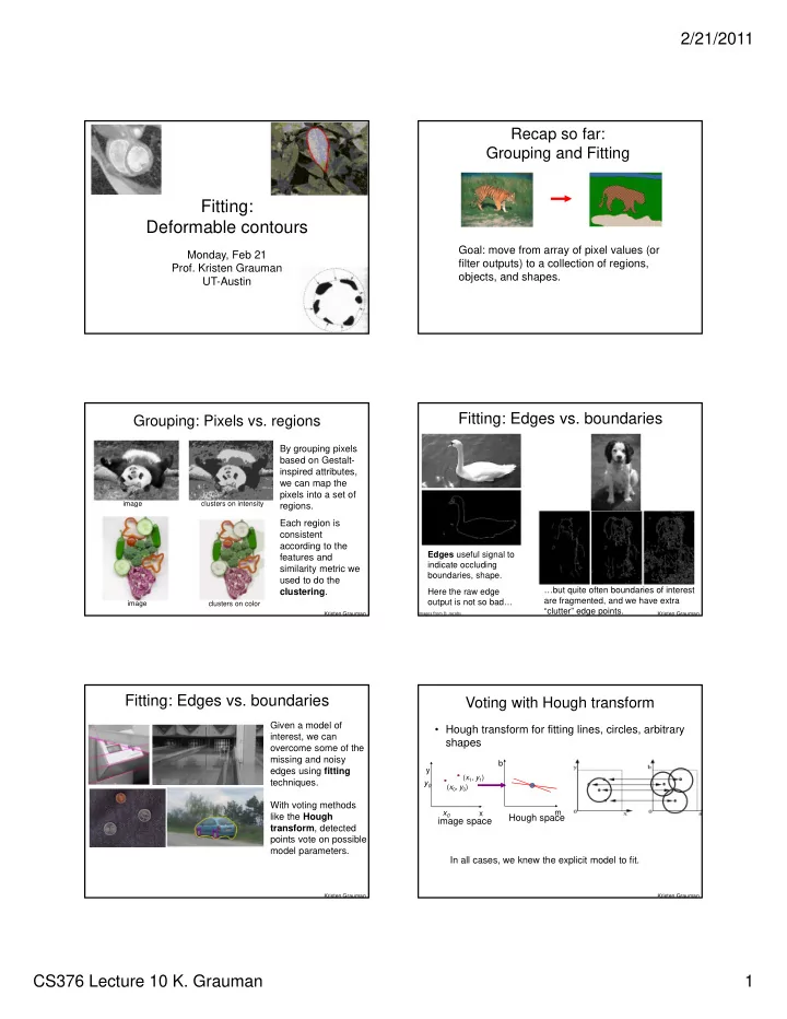
Fitting: Deformable contours
Monday, Feb 21
- Prof. Kristen Grauman
UT-Austin
Recap so far: Grouping and Fitting
Goal: move from array of pixel values (or filter outputs) to a collection of regions,
- bjects, and shapes.
Grouping: Pixels vs. regions
image clusters on intensity clusters on color image
By grouping pixels based on Gestalt- inspired attributes, we can map the pixels into a set of regions. Each region is consistent according to the features and similarity metric we used to do the clustering.
Kristen Grauman
Fitting: Edges vs. boundaries
Edges useful signal to indicate occluding boundaries, shape. Here the raw edge
- utput is not so bad…
…but quite often boundaries of interest are fragmented, and we have extra “clutter” edge points.
Images from D. Jacobs
Kristen Grauman
Given a model of interest, we can
- vercome some of the
missing and noisy edges using fitting techniques. With voting methods like the Hough transform, detected points vote on possible model parameters.
Fitting: Edges vs. boundaries
Kristen Grauman
Voting with Hough transform
- Hough transform for fitting lines, circles, arbitrary
shapes
x y
image space
x0 y0
(x0, y0) (x1, y1)
m b
Hough space In all cases, we knew the explicit model to fit.
Kristen Grauman