Fitting: Deformable contours Thurs Oct 1 Kristen Grauman UT - - PDF document

fitting deformable contours
SMART_READER_LITE
LIVE PREVIEW

Fitting: Deformable contours Thurs Oct 1 Kristen Grauman UT - - PDF document

9/30/2015 Fitting: Deformable contours Thurs Oct 1 Kristen Grauman UT Austin Recap so far: Grouping and Fitting Goal: move from array of pixel values (or filter outputs) to a collection of regions, objects, and shapes. Grouping: Pixels


slide-1
SLIDE 1

9/30/2015 1

Fitting: Deformable contours

Thurs Oct 1 Kristen Grauman UT Austin

Recap so far: Grouping and Fitting

Goal: move from array of pixel values (or filter outputs) to a collection of regions,

  • bjects, and shapes.

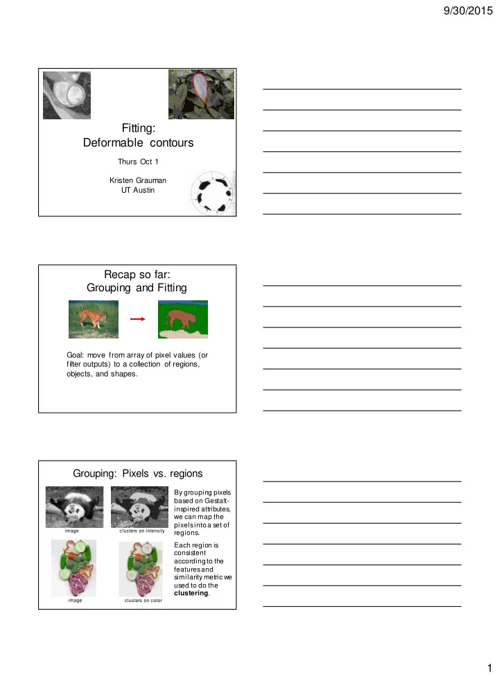
Grouping: Pixels vs. regions

image clusters on intensity clusters on color image

By grouping pixels based on Gestalt- inspired attributes, we can map the pixels into a set of regions. Each region is consistent according to the features and similarity metric we used to do the clustering.

slide-2
SLIDE 2

9/30/2015 2 Fitting: Edges vs. boundaries

Edges usef ul signal to indicate occluding boundaries, shape. Here the raw edge

  • utput is not so bad…

…but quite of ten boundaries of interest are f ragmented, and we hav e extra “clutter” edge points.

Images from D. Jacobs

Given a model of interest, we can

  • vercome some of the

missing and noisy edges using fitting techniques. With voting methods like the Hough transform, detected points vote on possible model parameters.

Fitting: Edges vs. boundaries

Voting with Hough transform

  • Hough transform for fitting lines, circles, arbitrary

shapes

x y

image space

x0 y0

(x0, y0) (x1, y1)

m b

Hough space In all cases, we knew the explicit model to fit.

slide-3
SLIDE 3

9/30/2015 3

  • Fitting an arbitrary shape w ith “active”

deformable contours

T

  • day

Deformable contours

a.k.a. active contours, snakes

Given: initial contour (model) near desired object

[Snakes: Active contour models, K ass, Witkin, & Terzopoulos, ICCV1987]

Figure credit: Yuri Boykov

Deformable contours

Given: initial contour (model) near desired object

a.k.a. active contours, snakes

Figure credit: Yuri Boykov

Goal: evolve the contour to fit exact object boundary

[Snakes: Active contour models, K ass, Witkin, & Terzopoulos, ICCV1987]

Main idea: elastic band is iteratively adjusted so as to

  • be near image positions with

high gradients, and

  • satisfy shape “preferences” or

contour priors

slide-4
SLIDE 4

9/30/2015 4

Deformable contours: intuition

Im age from http://www.healthlin e.c o m /blo gs /ex erc i s e_f itnes s /up loade d_im ages /HandBand2 -7 95868 .J PG

Deformable contours vs. Hough

initial intermediate final

Like generalized Hough transform, useful for shape fitting; but Hough Rigid model shape Single voting pass can detect multiple instances Deformable contours Prior on shape types, but shape iteratively adjusted (deforms) Requires initialization nearby One optimization “pass” to fit a single contour

Why do we want to fit deformable shapes?

  • Some objects have similar basic form but

some variety in the contour shape.

slide-5
SLIDE 5

9/30/2015 5

Why do we want to fit deformable shapes?

  • Non-rigid,

deformable

  • bjects can

change their shape over time, e.g. lips, hands…

Figure from Kass et al. 1987

Why do we want to fit deformable shapes?

  • Non-rigid,

deformable

  • bjects can

change their shape over time, e.g. lips, hands…

Figure credit: Julien Jomier

Why do we want to fit deformable shapes?

  • Non-rigid, deformable objects can change their shape
  • ver time.
slide-6
SLIDE 6

9/30/2015 6

Aspects we need to consider

  • Representation of the contours
  • Defining the energy functions

– External – Internal

  • Minimizing the energy function
  • Extensions:

– Tracking – Interactive segmentation

Representation

  • We’ll consider a discrete representation of the contour,

consisting of a list of 2d point positions (“vertices”).

), , (

i i i

y x   1 , , 1 ,   n i 

for

  • At each iteration, we’ll have the
  • ption to move each vertex to

another nearby location (“state”). ) , (

0 y

x ) , (

19 19 y

x

Fitting deformable contours

initial intermediate final

How should we adjust the current contour to form the new contour at each iteration?

  • Define a cost function (“energy” function) that says how

good a candidate configuration is.

  • Seek next configuration that minimizes that cost function.
slide-7
SLIDE 7

9/30/2015 7

Energy function

The total energy (cost) of the current snake is defined as:

external internal total

E E E  

A good fit between the current deformable contour and the target shape in the image will yield a low value for this cost function. Internal energy: encourage prior shape preferences: e.g., smoothness, elasticity, particular known shape. External energy (“image” energy): encourage contour to fit on places where image structures exist, e.g., edges.

External energy: intuition

  • Measure how well the curve matches the image data
  • “Attract” the curve toward different image features

– Edges, lines, texture gradient, etc.

External image energy

Magnitude of gradient

  • (Magnitude of gradient)

 

2 2

) ( ) ( I G I G

y x

 

2 2

) ( ) ( I G I G

y x

How do edges affect “snap” of rubber band? Think of external energy from image as gravitational pull towards areas of high contrast

slide-8
SLIDE 8

9/30/2015 8

  • Gradient images and
  • External energy at a point on the curve is:
  • External energy for the whole curve:

) , ( y x Gx ) , ( y x Gy

) | ) ( | | ) ( | ( ) (

2 2

  

y x external

G G E   

External image energy

2 1 2

| ) , ( | | ) , ( |

i i y n i i i x external

y x G y x G E

 

  

Internal energy: intuition

What are the underlying boundaries in this fragmented edge image? And in this one? A priori, we want to favor smooth shapes, contours with low curvature, contours similar to a known shape, etc. to balance what is actually observed (i.e., in the gradient image).

Internal energy: intuition

slide-9
SLIDE 9

9/30/2015 9 Internal energy

For a continuous curve, a common internal energy term is the “bending energy”. At some point v(s) on the curve, this is:

Tension, Elasticity Stiffness, Curvature

s d d ds d

s Einternal 2 2 )) ( (

2 2

 

    

  • For our discrete representation,
  • Internal energy for the whole curve:

1 ) , (    n i y x

i i i

 

i 1 i

v ds d    

 1 1 1 1 2 2

2 ) ( ) (

   

      

i i i i i i i

ds d        

    

    

1 2 1 1 2 1

2

n i i i i i i internal

E       

Internal energy

Note these are derivatives relative to position---not spatial image gradients. Why do these reflect tension and curvature?

Example: compare curvature

(1,1) (1,1) (2,2) (3,1) (3,1) (2,5)

2 1 1

2 ) (

 

  

i i i i curvature v

E   

3 − 2 2 + 1 2 + 1 − 2 5 + 1 2 3 − 2 2 + 1 2 + 1 − 2 2 + 1 2 = −8 2 = 64 = −2 2 = 4 2 1 1 2 1 1

) 2 ( ) 2 (

   

     

i i i i i i

y y y x x x

slide-10
SLIDE 10

9/30/2015 10 Penalizing elasticity

  • Current elastic energy definition uses a discrete estimate
  • f the derivative:

What is the possible problem with this definition?

2 1 1 2 1

) ( ) (

i i n i i i

y y x x     

   

   

1 2 1 n i i i elastic

E   

Penalizing elasticity

  • Current elastic energy definition uses a discrete estimate
  • f the derivative:

   

1 2 1 n i i i elastic

E   

 

2 1 2 1 2 1

) ( ) (

   

     

n i i i i i

d y y x x 

where d is the average distance between pairs of points – updated at each iteration.

Instead:

Dealing with missing data

  • The preferences for low-curvature, smoothness help

deal with missing data:

[Figure from Kass et al. 1987]

Illusory contours found!

slide-11
SLIDE 11

9/30/2015 11 Extending the internal energy: capture shape prior

  • If object is some smooth variation on a

known shape, we can use a term that will penalize deviation from that shape: where are the points of the known shape.

 

   

1 2

) ˆ (

n i i i internal

E   

} ˆ {

i

Fig from Y . Boykov

Total energy: function of the weights

external internal total

E E E     

    

     

1 2 1 1 2 1

2

n i i i i i i internal

d E       

2 1 2

| ) , ( | | ) , ( |

i i y n i i i x external

y x G y x G E

 

  

large  small  medium 

  • e.g., weight controls the penalty for internal elasticity

Fig from Y . Boykov

Total energy: function of the weights

slide-12
SLIDE 12

9/30/2015 12 Recap: deformable contour

  • A simple elastic snake is defined by:

– A set of n points, – An internal energy term (tension, bending, plus optional shape prior) – An external energy term (gradient-bas ed)

  • To use to segment an object:

– Initialize in the vicinity of the object – Modify the points to minimize the total energy

Energy minimization

  • Several algorithms have been proposed to fit

deformable contours.

  • We’ll look at tw o:

– Greedy search – Dynamic programming (for 2d snakes)

Energy minimization: greedy

  • For each point, search window around

it and move to where energy function is minimal

– Typical window size, e.g., 5 x 5 pixels

  • Stop when predefined number of

points have not changed in last iteration, or after max number of iterations

  • Note:

– Convergence not guaranteed – Need decent initialization

slide-13
SLIDE 13

9/30/2015 13 Energy minimization

  • Several algorithms have been proposed to fit

deformable contours.

  • We’ll look at tw o:

– Greedy search – Dynamic programming (for 2d snakes)

1

v

2

v

3

v

4

v

6

v

5

v With this form of the energy function, we can minimize using dynamic programming, with the Viterbi algorithm. Iterate until optimal position for each point is the center

  • f the box, i.e., the snake is optimal in the local search

space constrained by boxes.

)

 

   

[Amini, Weymouth, Jain, 1990]

   

     

Fig from Y . Boykov

Energy minimization: dynamic programming Energy minimization: dynamic programming

  

1 1 1 1

) , ( ) , , (

n i i i i n total

E E     

  • Possible because snake energy can be rewritten as a

sum of pair-wise interaction potentials:

  • Or sum of triple-interaction potentials.

   

1 1 1 1 1

) , , ( ) , , (

n i i i i i n total

E E      

slide-14
SLIDE 14

9/30/2015 14 Snake energy: pair-wise interactions

2 1 1 2 1 1

| ) , ( | | ) , ( | ) , , , , , (

i i y n i i i x n n total

y x G y x G y y x x E

 

    

2 1 1 1 2 1

) ( ) (

i i n i i i

y y x x     

   

 

 

1 1 2 1

|| ) ( || ) , , (

n i i n total

G E    

   

 

1 1 2 1

|| ||

n i i i

   ) , ( ... ) , ( ) , ( ) , , (

1 1 3 2 2 2 1 1 1 n n n n total

v v E v v E v v E E

 

      

2 1 2 1

|| || || ) ( || ) , (

i i i i i i

G E          

 

where

Re-writing the above with :

 

i i i

y x v ,  ) , (

4 4 n

v v E ) , (

4 3 3

v v E ) 3 (

3

E ) (

3 m

E ) (

4 m

E ) 3 (

4

E ) 2 (

4

E ) 1 (

4

E ) (m En ) 3 (

n

E ) 2 (

n

E ) 1 (

n

E ) 2 (

3

E ) 1 (

3

E ) (

2 m

E ) 3 (

2

E

) , ( ... ) , ( ) , (

1 1 3 2 2 2 1 1 n n n total

v v E v v E v v E E

 

   

) , (

3 2 2

v v E ) 1 (

2

E ) 2 (

2

E ) , (

2 1 1

v v E ) 1 (

1

 E ) 2 (

1

 E ) 3 (

1

 E ) (

1

 m E

Main idea: determine optimal position (state) of predecessor, for each possible position of self. Then backtrack from best state for last vertex.

states 1 2 … m vertices

1

v

2

v

3

v

4

v

n

v

) (

2

nm O

Complexity:

  • vs. brute force search ____?

Viterbi algorithm

Example adapted from Y . Boykov

1

v

2

v

3

v

4

v

6

v

5

v With this form of the energy function, we can minimize using dynamic programming, with the Viterbi algorithm. Iterate until optimal position for each point is the center

  • f the box, i.e., the snake is optimal in the local search

space constrained by boxes.

[Amini, Weymouth, Jain, 1990] Fig from Y . Boykov

Energy minimization: dynamic programming

slide-15
SLIDE 15

9/30/2015 15

) , ( ... ) , ( ) , (

1 1 3 2 2 2 1 1 n n n

v v E v v E v v E

 

  

DP can be applied to optimize an open ended snake For a closed snake, a “loop” is introduced into the total energy.

1

n

) , ( ) , ( ... ) , ( ) , (

1 1 1 3 2 2 2 1 1

v v E v v E v v E v v E

n n n n n

   

 

1

n

2

1  n

3

4

Work around: 1) Fix v1 and solve for rest . 2) Fix an intermediate node at its position found in (1), solve for rest.

Energy minimization: dynamic programming

Aspects we need to consider

  • Representation of the contours
  • Defining the energy functions

– External – Internal

  • Minimizing the energy function
  • Extensions:

– Tracking – Interactive segmentation

Tracking via deformable contours

  • 1. Use final contour/model extracted at frame t as

an initial solution for frame t+1

  • 2. Evolve initial contour to fit exact object boundary

at frame t+1

  • 3. Repeat, initializing with most recent frame.

Tracking Heart Ventricles (multiple frames)

slide-16
SLIDE 16

9/30/2015 16

Visual Dynamics Group, Dept. Engineering Science, University of Oxf

  • rd.

Traffic monitoring Human-computer interaction Animation Surveillance Computer assisted diagnosis in medical imaging Applications:

Tracking via deformable contours

3D active contours

  • Jörgen Ahlberg
  • http://www.cvl.isy.liu.se/ScOut/M

asters/Papers/E x1708.pdf

  • May over-smooth the boundary
  • Cannot follow topological changes of objects

Limitations

slide-17
SLIDE 17

9/30/2015 17

Limitations

  • External energy: snake does not really “see” object

boundaries in the image unless it gets very close to it.

image gradients are large only directly on the boundary

I 

Distance transform

  • External image can instead be taken from the distance

transform of the edge image.

  • riginal
  • gradient

distance transform edges

V alue at (x,y) tells how far that position is from the nearest edge point (or other binary mage structure)

>> help bwdist

Interactive forces

How can we implement such an interactive force with deformable contours?

slide-18
SLIDE 18

9/30/2015 18

Interactive forces

  • An energy function can be altered online based
  • n user input – use the cursor to push or pull the

initial snake aw ay from a point.

  • Modify external energy term to include:

 

 

1 2 2

| |

n i i push

p r E 

Nearby points get pushed hardest

Intelligent scissors

[Mortensen & Barrett, SIGGRAPH 1995, CVPR 1999]

Another form of interactive segmentation: Compute optimal paths from every point to the seed based on edge-related costs.

  • http://rivit.cs.byu.edu/Eric/Eric.html

Intelligent scissors

slide-19
SLIDE 19

9/30/2015 19

  • http://rivit.cs.byu.edu/Eric/Eric.html

Intelligent scissors

Deformable contours: pros and cons

Pros:

  • Useful to track and fit non-rigid shapes
  • Contour remains connected
  • Possible to fill in “subjective” contours
  • Flexibility in how energy function is defined, weighted.

Cons:

  • Must have decent initialization near true boundary, may

get stuck in local minimum

  • Parameters of energy function must be set well bas

ed on prior information

Summary

  • Deformable shapes and active contours are useful for

– Segmentation: fit or “snap” to boundary in image – Tracking: previous frame’s estimate serves to initialize the next

  • Fitting active contours:

– Define terms to encourage certain shapes, smoothness, low curvature, push/pulls, … – Use weights to control relative influence of each component cost – Can optimize 2d snakes with Viterbi algorithm.

  • Image structure (esp. gradients) can act as attraction

force for interactivesegmentation methods.