
SLIDE 1 Over fitting
and
Under
fitting
- Under
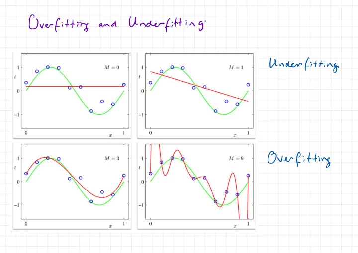
Over fitting distribution functions over Bayesian Regression / - - PowerPoint PPT Presentation
Over fitting Under fitting and - Under fitting Over fitting distribution functions over Bayesian Regression / " ' i diggllloise dist ' f. fnpc f) fcxn ) - ,N En n=1 + En~ PIE yn = ... , of Basis Function
"
' i 'diggllloise
dist yn = fcxn ) + En fnpc f) En~ PIE n=1 , ... ,N Linear Basis Function×=tI÷El}
"t.ae#=t9tEIII1NX1NxDpxl
[ TEI
= IF cyn . wto .it +ia¥
, wa ' I = ETE
)Often
) t En Wd ~ Norm ( o , 5) En £
, yn . ¢⇒ ) ' +,n=
Maximum a Posteriori Estimation yn = ITw--oThi
Distribution
gf
y
Informal Definition...
h( × ,× ' ) Covariance function fcx) .YnIF=f~
Norm ( f IIn
) ,6 ) i=
µ 1£ ) Prior acx.xx.gg)
be CX , X ) h ( x ' ,X* I M Xl M X N MX M pic x ) = ( ME ) , . . . , pika ) ) thx "t.lu#xlhcx:xmtotD
lil
" Probability density for jointly Gaussian variables N N MXN NXM ZE RN pie , f) = Normtil
:/
, 1¥81 ) perm M M ur xN MXM Marginals poet = Norm a- , A ) pcp's = Norm (p ;D B ) next ' N XX I N x I Conditional pip If ) = Norm 1/5 ; b- *
tuft
:
"i¥lK¥
":&
:¥¥÷D
B b- c D PredictiveI
i=
µ 1£ ) Prior ELY
) = OIK)Efw
] = OI (Xo ) mo = tell ) Cov [ 4 ] = Cov I IK ) w ] t 62 I = IN Covlw ] # I Xlt + 62 I µ xD Dxb DX N = ④ G) So # HT t 6- I = kk ,Nt5I . OIKIW
, EI ) W titty
Complexity :0447=011×9
# KIT ( Ik ) # Cx)Ttg÷I5' y OCD ) = OI Htt ) ( OI KY # K ) + III ) " It Cxlty Conclusion : Posterior mean equivalent to Ridge Regression In
,In
) = § Old (In
) So.de/0eCXm
) functor implies e choice .fr/Vonm(k(xIx)lklx.xlto2IYy
k(x4x* ) increases
with67
and decreases with weightvariances
' Gaussian Processes : . y # rIdf
ply 'Tf) plfly )