Outline Fitting Surfaces to Very Large Meshes Multiresolution - PDF document

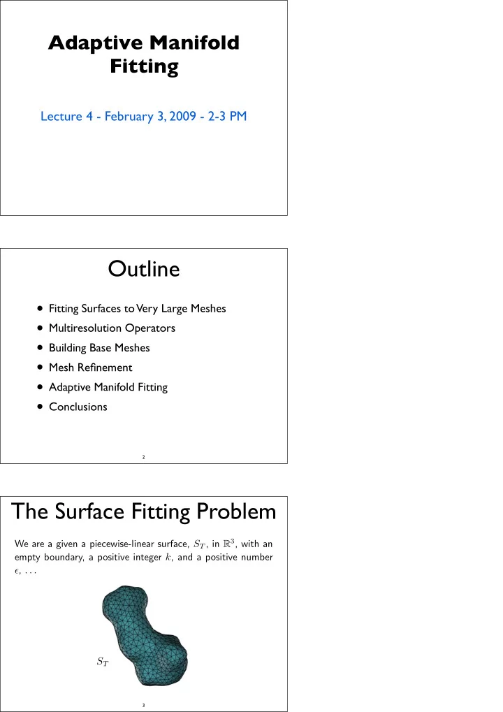
Adaptive Manifold Fitting Lecture 4 - February 3, 2009 - 2-3 PM Outline • Fitting Surfaces to Very Large Meshes • Multiresolution Operators • Building Base Meshes • Mesh Refinement • Adaptive Manifold Fitting • Conclusions 2 The Surface Fitting Problem We are a given a piecewise-linear surface, S T , in R 3 , with an empty boundary, a positive integer k , and a positive number � , . . . S T 3

The Surface Fitting Problem We want to find a C k surface S ⊂ R 3 . . . S ⊂ R 3 4 The Surface Fitting Problem such that there exists a homeomorphism, h : S → | S T | , satis- fying � h ( v ) − v � ≤ � , for every vertex v of S T . 5 Surface Fitting • Very Large Meshes (10 6 vertices) - Challenging Problem! 6

Manifolds and Fitting • Basic Setting - Gluing Data proportional to Mesh Size • Problem: Very Large Meshes - Computationally Inefficient - Do not Exploit Approximation Power • Solution: - Adaptation 7 Adaptive Fitting • Optimization Formulation: - Given an Approximation Error - Find with Smallest Number of Charts • Strategy: - Combine Multiresolution Structure • Manifold Surface Approximation • 8 Multiresolution Framework • Simplicial Multi-triangulation - Stellar Theory • Building Base Meshes - Surface Simplification • Adaptive Fitting - 4-8 Refinement 9

Stellar Theory • Topological Operators • Edge Split and Weld - Change Mesh Resolution • Edge Flip - Change Mesh Connectivity 10 Stellar Simplification • Basic Elements: I. Operator Factorization - Edge Collapse - Flip + Weld II. Quadric Error Metric 11 Basic Algorithm • Repeat for N Resolution Levels 1. Rank Vertices Based on Quadric Error 2. Select Independent Set of Clusters 3. Simplify Mesh using Stellar Operators ✴ Properties - Logarithmic Height - Good Aspect Ratios 12

Example 1: Plane 13 Example 2: Cow 14 Variable Resolution Mesh • Underlying Semi-Regular Structure - Tri-quad Base Mesh - 4-8 Subdivision 15

Building the Base Mesh 1. Two-Face Clusters + Single Triangles 2. Barycenter Subdivision 16 4-8 Subdivision • Interleaved Binary Subdivision i i+1 i+2 • Non-Uniform Refinement 17 Binary Multi-Triangulation Base Mesh Edge Splits 18

Adaptive Refinement 19 Example I: Uniform 20 Example 2: Adaptive • Application-Dependent Criteria Spatial Selection Curvature 21

Adaptive Fitting S T PIPELINE ˜ S T = Simplify S T Embed ˜ S T in | S T | Refine ˜ S T Create S from ˜ S T S 22 Adaptive Fitting ˜ S T S T = Simplify S T • Four-Face Clusters Algorithm S T ˜ S T 23 Adaptive Fitting Embed ˜ S T in | S T | • Each edge of ˜ S T is embedded in | S T | as a “geodesic”. S T ˜ S T 24

Adaptive Fitting REMARK : The vertices of ˜ S T ARE vertices of S T . S T ˜ S T 25 Adaptive Fitting Create S from ˜ S T • For each vertex v of ˜ S T , we consider the P-polygon, P v , of v in R 2 , and the standard triangulation, T v , of the P-polygon P v . v s v ( v ) ˜ S T T v 26 Adaptive Fitting Create S from ˜ S T • Consider the embedding of the star, st ( v, ˜ S T ) , of v in S T . S T 27

Adaptive Fitting Create S from ˜ S T • Map the vertices of S T bounded by the embedding of st ( v, ˜ S T ) to T v . w w σ v v u ˜ S T u S T 28 Adaptive Fitting Create S from ˜ S T • Map the vertices of S T bounded by the embedding of st ( v, ˜ S T ) to T v . w s v ( w ) s v ( σ ) s v ( u ) v s v ( v ) T v u S T 29 Adaptive Fitting Create S from ˜ S T • Map the vertices of S T bounded by the embedding of st ( v, ˜ S T ) to T v . w s v ( w ) s v ( u ) v s v ( v ) T v u S T 30

Adaptive Fitting Create S from ˜ S T • We map the vertices in each “curved” triangle sepa- rately. w “curved triangle” v u S T 31 Adaptive Fitting Create S from ˜ S T • We use Floater’s parametrization to build the map for each ”curved” triangle. s v ( w ) w v s v ( v ) s v ( u ) u S T 32 Adaptive Fitting Create S from ˜ S T • For each triangle in st ( v, ˜ S T ) , compute the shape func- tion ψ v . b 01 b 11 2 b 21 1.5 1 1 y b 22 0.5 0 0 0 4 4 0 b 00 3 3 1 2 2 2 z z x b 10 1 1 3 0 0 4 b 20 33

Adaptive Fitting Create S from ˜ S T • Control points of ψ v are computed by a least squares procedure. • But, this time, the sample points are the vertices of S T that correspond to the points in T v through Floater’s parametrization! 34 Adaptive Fitting Create S from ˜ S T • For each point p ∈ T v , we compute the approximation error , � q − ψ v ( p ) � , where q is the vertex of S T corresponding to p through Floater’s parametrization. • If the above error is smaller than the given number � , we keep computing ψ u , for each u ∈ I . Otherwise, we stop this process and go to the refinement step. 35 Adaptive Fitting Refine ˜ S T • We locally refine ˜ S T using the stellar operations and the 4-8 refinement, and then embed the resulting ˜ S T in | S T | again. Embed ˜ S T in | S T | Refine ˜ S T Create S from ˜ S T 36

Conclusions • Simplicial Multiresolution - Powerful Mechanism for Adaptation • First Part - Simplification - Adaptive Refinement • Second Part - Geodesic Parametrization - Bezier Approximation 37