Myself Researcher at CNR-IMATI & Member of the Shape and - - PowerPoint PPT Presentation

SLIDE 1

Laplacian Spectral Functions, Kernels, and Distances

Theory & Applications to Geometry Processing & Shape Analysis

Giuseppe Patanè CNR-IMATI, Genova - Italy

patane@ge.imati.cnr.it

Myself

• Researcher at CNR-IMATI & Member of the “Shape and Seman<cs Modelling

Group” (since 2001)

• Responsible of the research line “Numerical Geometry and Signal Processing”
• NaHonal ScienHfic HabilitaHon

– Full Professor in Computer Science (INF01) – Full Professor in Systems for Informa3on Processing (ENG-09/H1)

• My research and training interests lie at the intersec<on of

– Computer Science: Computer Graphics & Mul<media, Machine Learning – Engineering: Informa<on & Signal Processing – Applied MathemaHcs: Numerical Analysis

• ERC Sector: PE6 Computer Science & InformaHcs

IntroducHon

Geometric & Topological approaches FuncHonal approaches

Shape Descriptors FuncHons, Kernels & Distances

Remeshing/skeletonisa<on/segmenta<on/etc

ApplicaHons

IntroducHon

FuncHonal approaches Laplacian spectral approaches

(∆, ϕ)

Remeshing/skeletonisa<on/segmenta<on/etc

ApplicaHons

Laplacian & Hamiltonian spectral funcHons

• Harmonic func<ons
• Laplacian/Hamiltonian

eigenfunc<ons

• Diffusive func<ons

Laplacian spectral funcHons, kernels & distances

Laplacian spectral kernels and distances

• Commute <me &

biharmonic

• Diffusion & wave
• …

SLIDE 2

• Target properHes of the Laplacian spectral

func<ons, kernels, and distances –smoothness & orthonormality –intrinsic definiHon; ie., independent of data embedding/representa<on –mulH-scale definiHon, in order to encode local and global shape features –invariance to shape transformaHons; eg., isometries for pose invariance –compact support & localisaHon at feature/ seed points for encoding local geometry proper<es & saving memory space –efficient, stable, and parameter-free computaHon

Different resoluHons Different & parHal representaHons Different postures

IntroducHon IntroducHon

• Working on the space of scalar funcHons defined on the input domain (eg., surface,

volume), we can address – mulH-scale signal representaHons and denoising, by projec<ng the input signals/data on a set of (mul3-scale) basis func<ons – sparse representaHons, by choosing a low number of basis func<ons in order to achieve a target approxima<on accuracy – compression, by quan<sing the representa<on coefficients MulH-scale/sparse representaHon Compression

f =

k

X

i=1

αiϕi

k = 3, 20, 50, . . .

f = (x, y, z)

IntroducHon

• Working on the space of scalar funcHons defined on the input domain (eg., surface,

volume), we can address – shape deformaHons, by modifying the coefficients that express the geometry of the input surface in terms of geometry-driven or shape-intrinsic basis funcHons (eg., harmonic barycentric coordinates)

f = X

i

αi(t)ϕi

Global basis Local basis

IntroducHon

• Working on the space of scalar funcHons defined on the input domain (eg., surface,

volume), we can address – the defini<on of Laplacian spectral kernels and distances, as a filtered combina<on of the Laplacian spectral basis

d2(p, q) := X

i

αi|ϕi(p) − ϕi(q)|2

seed point

p

<latexit sha1_base64="TxjeQN1S0yLSUh93TOGy+Iti9rM=">AB8HicbVBNS8NAFHypX7V+VT16WSyCp5KIoN6KXjxWMLbYlrLZvrRLN5uwuxFK6L/w4kHFqz/Hm/GTZuDtg4sDPvsfMmSATXxnW/ndLK6tr6RnmzsrW9s7tX3T940HGqGPosFrFqB1Sj4BJ9w43AdqKQRoHAVjC+yf3WEyrNY3lvJgn2IjqUPOSMGis9diNqRkGYJdN+tebW3RnIMvEKUoMCzX71qzuIWRqhNExQrTuem5heRpXhTOC0k01JpSN6RA7lkoaoe5ls8RTcmKVAQljZ80ZKb+3shopPUkCuxknlAvern4n9dJTXjZy7hMUoOSzT8KU0FMTPLzyYArZEZMLKFMcZuVsBFVlBlbUsW4C2evEz8s/pV3bs7rzWuizbKcATHcAoeXEADbqEJPjCQ8Ayv8OZo58V5dz7moyWn2DmEP3A+fwBbsJDo</latexit><latexit sha1_base64="TxjeQN1S0yLSUh93TOGy+Iti9rM=">AB8HicbVBNS8NAFHypX7V+VT16WSyCp5KIoN6KXjxWMLbYlrLZvrRLN5uwuxFK6L/w4kHFqz/Hm/GTZuDtg4sDPvsfMmSATXxnW/ndLK6tr6RnmzsrW9s7tX3T940HGqGPosFrFqB1Sj4BJ9w43AdqKQRoHAVjC+yf3WEyrNY3lvJgn2IjqUPOSMGis9diNqRkGYJdN+tebW3RnIMvEKUoMCzX71qzuIWRqhNExQrTuem5heRpXhTOC0k01JpSN6RA7lkoaoe5ls8RTcmKVAQljZ80ZKb+3shopPUkCuxknlAvern4n9dJTXjZy7hMUoOSzT8KU0FMTPLzyYArZEZMLKFMcZuVsBFVlBlbUsW4C2evEz8s/pV3bs7rzWuizbKcATHcAoeXEADbqEJPjCQ8Ayv8OZo58V5dz7moyWn2DmEP3A+fwBbsJDo</latexit><latexit sha1_base64="TxjeQN1S0yLSUh93TOGy+Iti9rM=">AB8HicbVBNS8NAFHypX7V+VT16WSyCp5KIoN6KXjxWMLbYlrLZvrRLN5uwuxFK6L/w4kHFqz/Hm/GTZuDtg4sDPvsfMmSATXxnW/ndLK6tr6RnmzsrW9s7tX3T940HGqGPosFrFqB1Sj4BJ9w43AdqKQRoHAVjC+yf3WEyrNY3lvJgn2IjqUPOSMGis9diNqRkGYJdN+tebW3RnIMvEKUoMCzX71qzuIWRqhNExQrTuem5heRpXhTOC0k01JpSN6RA7lkoaoe5ls8RTcmKVAQljZ80ZKb+3shopPUkCuxknlAvern4n9dJTXjZy7hMUoOSzT8KU0FMTPLzyYArZEZMLKFMcZuVsBFVlBlbUsW4C2evEz8s/pV3bs7rzWuizbKcATHcAoeXEADbqEJPjCQ8Ayv8OZo58V5dz7moyWn2DmEP3A+fwBbsJDo</latexit><latexit sha1_base64="TxjeQN1S0yLSUh93TOGy+Iti9rM=">AB8HicbVBNS8NAFHypX7V+VT16WSyCp5KIoN6KXjxWMLbYlrLZvrRLN5uwuxFK6L/w4kHFqz/Hm/GTZuDtg4sDPvsfMmSATXxnW/ndLK6tr6RnmzsrW9s7tX3T940HGqGPosFrFqB1Sj4BJ9w43AdqKQRoHAVjC+yf3WEyrNY3lvJgn2IjqUPOSMGis9diNqRkGYJdN+tebW3RnIMvEKUoMCzX71qzuIWRqhNExQrTuem5heRpXhTOC0k01JpSN6RA7lkoaoe5ls8RTcmKVAQljZ80ZKb+3shopPUkCuxknlAvern4n9dJTXjZy7hMUoOSzT8KU0FMTPLzyYArZEZMLKFMcZuVsBFVlBlbUsW4C2evEz8s/pV3bs7rzWuizbKcATHcAoeXEADbqEJPjCQ8Ayv8OZo58V5dz7moyWn2DmEP3A+fwBbsJDo</latexit>

q

<latexit sha1_base64="meX57DK1w2i7CaTi1VTDOai/VSY=">AB8HicbVBNS8NAFHzxs9avqkcvi0XwVBIR1FvRi8cKxhbUjbTbt0s4m7L0IJ/RdePKh49ed489+4aXPQ1oGFYeY9dt4EiRQGXfbWVpeWV1bL2UN7e2d3Yre/v3Jk414z6LZaxbATVcCsV9FCh5K9GcRoHkzWB0nfvNJ6NiNUdjhPejehAiVAwilZ6EQUh0GYPU56lapbc6cgi8QrSBUKNHqVr04/ZmnEFTJjWl7boLdjGoUTPJuZManlA2ogPetlTRiJtuNk08IcdW6ZMw1vYpJFP190ZGI2PGUWAn84Rm3svF/7x2iuFNxMqSZErNvsoTCXBmOTnk7QnKEcW0KZFjYrYUOqKUNbUtmW4M2fvEj809plzbs9q9avijZKcAhHcAIenEMdbqABPjBQ8Ayv8OY58V5dz5mo0tOsXMAf+B8/gBdNJDp</latexit><latexit sha1_base64="meX57DK1w2i7CaTi1VTDOai/VSY=">AB8HicbVBNS8NAFHzxs9avqkcvi0XwVBIR1FvRi8cKxhbUjbTbt0s4m7L0IJ/RdePKh49ed489+4aXPQ1oGFYeY9dt4EiRQGXfbWVpeWV1bL2UN7e2d3Yre/v3Jk414z6LZaxbATVcCsV9FCh5K9GcRoHkzWB0nfvNJ6NiNUdjhPejehAiVAwilZ6EQUh0GYPU56lapbc6cgi8QrSBUKNHqVr04/ZmnEFTJjWl7boLdjGoUTPJuZManlA2ogPetlTRiJtuNk08IcdW6ZMw1vYpJFP190ZGI2PGUWAn84Rm3svF/7x2iuFNxMqSZErNvsoTCXBmOTnk7QnKEcW0KZFjYrYUOqKUNbUtmW4M2fvEj809plzbs9q9avijZKcAhHcAIenEMdbqABPjBQ8Ayv8OY58V5dz5mo0tOsXMAf+B8/gBdNJDp</latexit><latexit sha1_base64="meX57DK1w2i7CaTi1VTDOai/VSY=">AB8HicbVBNS8NAFHzxs9avqkcvi0XwVBIR1FvRi8cKxhbUjbTbt0s4m7L0IJ/RdePKh49ed489+4aXPQ1oGFYeY9dt4EiRQGXfbWVpeWV1bL2UN7e2d3Yre/v3Jk414z6LZaxbATVcCsV9FCh5K9GcRoHkzWB0nfvNJ6NiNUdjhPejehAiVAwilZ6EQUh0GYPU56lapbc6cgi8QrSBUKNHqVr04/ZmnEFTJjWl7boLdjGoUTPJuZManlA2ogPetlTRiJtuNk08IcdW6ZMw1vYpJFP190ZGI2PGUWAn84Rm3svF/7x2iuFNxMqSZErNvsoTCXBmOTnk7QnKEcW0KZFjYrYUOqKUNbUtmW4M2fvEj809plzbs9q9avijZKcAhHcAIenEMdbqABPjBQ8Ayv8OY58V5dz5mo0tOsXMAf+B8/gBdNJDp</latexit><latexit sha1_base64="meX57DK1w2i7CaTi1VTDOai/VSY=">AB8HicbVBNS8NAFHzxs9avqkcvi0XwVBIR1FvRi8cKxhbUjbTbt0s4m7L0IJ/RdePKh49ed489+4aXPQ1oGFYeY9dt4EiRQGXfbWVpeWV1bL2UN7e2d3Yre/v3Jk414z6LZaxbATVcCsV9FCh5K9GcRoHkzWB0nfvNJ6NiNUdjhPejehAiVAwilZ6EQUh0GYPU56lapbc6cgi8QrSBUKNHqVr04/ZmnEFTJjWl7boLdjGoUTPJuZManlA2ogPetlTRiJtuNk08IcdW6ZMw1vYpJFP190ZGI2PGUWAn84Rm3svF/7x2iuFNxMqSZErNvsoTCXBmOTnk7QnKEcW0KZFjYrYUOqKUNbUtmW4M2fvEj809plzbs9q9avijZKcAhHcAIenEMdbqABPjBQ8Ayv8OY58V5dz5mo0tOsXMAf+B8/gBdNJDp</latexit>

SLIDE 3

IntroducHon

• Working on the space of scalar funcHons defined on the input domain (eg., surface,

volume), we can address – shape correspondence and comparison, by expressing the problem with respect to a basis and conver<ng it to a linear or least-squares problem

p q

T : M → N δp

FT (δp) ≈ δq

FT : F(M) → F(N)

Goals

• Review of previous work on the defini<on, discre<sa<on, and

computa<on of Laplacian & Hamiltonian spectral funcHons – harmonic func<ons – Laplacian/Hamiltonian eigenfunc<ons – diffusive func<ons, as solu<ons to the heat equa<on – …

Harmonic funcHon Diffusive funcHons at different scales

. . .

<latexit sha1_base64="M7GmIEvNqbUz4Gtf8JvV+IicJ18=">AB7HicbVBNS8NAEJ34WetX1aOXYBE8lUQE9Vb04rGCaQtKJvNpl272Q27E6GU/gcvHlS8+oO8+W/ctjlo64OBx3szMyLMsENet63s7K6tr6xWdoqb+/s7u1XDg6bRuWasoAqoXQ7IoYJLlmAHAVrZ5qRNBKsFQ1vp37riWnDlXzAUcbClPQlTzglaKVmV8QKTa9S9WreDO4y8QtShQKNXuWrGyuap0wiFcSYju9lGI6JRk4Fm5S7uWEZoUPSZx1LJUmZCcezayfuqViN1HalkR3pv6eGJPUmFEa2c6U4MAselPxP6+TY3IVjrnMcmSzhcluXBRudPX3ZhrRlGMLCFUc3urSwdE4o2oLINwV98eZkE57Xrmn9/Ua3fFGmU4BhO4Ax8uIQ63EDAqDwCM/wCm+Ocl6cd+dj3riFDNH8AfO5w8odo8M</latexit><latexit sha1_base64="M7GmIEvNqbUz4Gtf8JvV+IicJ18=">AB7HicbVBNS8NAEJ34WetX1aOXYBE8lUQE9Vb04rGCaQtKJvNpl272Q27E6GU/gcvHlS8+oO8+W/ctjlo64OBx3szMyLMsENet63s7K6tr6xWdoqb+/s7u1XDg6bRuWasoAqoXQ7IoYJLlmAHAVrZ5qRNBKsFQ1vp37riWnDlXzAUcbClPQlTzglaKVmV8QKTa9S9WreDO4y8QtShQKNXuWrGyuap0wiFcSYju9lGI6JRk4Fm5S7uWEZoUPSZx1LJUmZCcezayfuqViN1HalkR3pv6eGJPUmFEa2c6U4MAselPxP6+TY3IVjrnMcmSzhcluXBRudPX3ZhrRlGMLCFUc3urSwdE4o2oLINwV98eZkE57Xrmn9/Ua3fFGmU4BhO4Ax8uIQ63EDAqDwCM/wCm+Ocl6cd+dj3riFDNH8AfO5w8odo8M</latexit><latexit sha1_base64="M7GmIEvNqbUz4Gtf8JvV+IicJ18=">AB7HicbVBNS8NAEJ34WetX1aOXYBE8lUQE9Vb04rGCaQtKJvNpl272Q27E6GU/gcvHlS8+oO8+W/ctjlo64OBx3szMyLMsENet63s7K6tr6xWdoqb+/s7u1XDg6bRuWasoAqoXQ7IoYJLlmAHAVrZ5qRNBKsFQ1vp37riWnDlXzAUcbClPQlTzglaKVmV8QKTa9S9WreDO4y8QtShQKNXuWrGyuap0wiFcSYju9lGI6JRk4Fm5S7uWEZoUPSZx1LJUmZCcezayfuqViN1HalkR3pv6eGJPUmFEa2c6U4MAselPxP6+TY3IVjrnMcmSzhcluXBRudPX3ZhrRlGMLCFUc3urSwdE4o2oLINwV98eZkE57Xrmn9/Ua3fFGmU4BhO4Ax8uIQ63EDAqDwCM/wCm+Ocl6cd+dj3riFDNH8AfO5w8odo8M</latexit><latexit sha1_base64="M7GmIEvNqbUz4Gtf8JvV+IicJ18=">AB7HicbVBNS8NAEJ34WetX1aOXYBE8lUQE9Vb04rGCaQtKJvNpl272Q27E6GU/gcvHlS8+oO8+W/ctjlo64OBx3szMyLMsENet63s7K6tr6xWdoqb+/s7u1XDg6bRuWasoAqoXQ7IoYJLlmAHAVrZ5qRNBKsFQ1vp37riWnDlXzAUcbClPQlTzglaKVmV8QKTa9S9WreDO4y8QtShQKNXuWrGyuap0wiFcSYju9lGI6JRk4Fm5S7uWEZoUPSZx1LJUmZCcezayfuqViN1HalkR3pv6eGJPUmFEa2c6U4MAselPxP6+TY3IVjrnMcmSzhcluXBRudPX3ZhrRlGMLCFUc3urSwdE4o2oLINwV98eZkE57Xrmn9/Ua3fFGmU4BhO4Ax8uIQ63EDAqDwCM/wCm+Ocl6cd+dj3riFDNH8AfO5w8odo8M</latexit>

Laplacian eigen-funcHons at different frequencies

Goals

• Review of previous work on the defini<on, discre<sa<on, and

computa<on of Laplacian spectral kernels and distances (eg. commute <me, biharmonic, wave kernel distances) by – filtering the Laplacian spectrum – generalising results on the heat diffusion kernels and distances.

Bi-harmonic dist. Diffusion dist. Mexican hat dist.

Goals

• Our review will be “independent” of

– data dimensionality (surface, volume, nD data) – discre<sa<on of the input domain (mesh, point set) and the Laplace-Beltrami operator

SLIDE 4

Goals

• Analysis of preview work on the computa<on of the Laplacian

spectral func<ons, kernels, and distances in terms of – robustness with respect to the discre<sa<on of the input domain: connec<vity, sampling, and smoothness (eg. geometric/topological noise)

Goals

• Analysis of preview work on the computa<on of the Laplacian

spectral func<ons, kernels, and distances in terms of – numerical proper<es (eg., sparsity, condi<oning number) of the Laplacian matrix and filter behaviour

Goals

• Analysis of preview work on the computa<on of the Laplacian

spectral func<ons, kernels, and distances in terms of – numerical accuracy/stability: convergence, Gibbs phen. – computa<onal cost & storage overhead – selec<on of parameters & heuris<cs

Goals

3D Shape

M

n points

. . .

Space of scalar funcHons defined on M

Φ ∈ Rn×n

• In the space of scalar func<ons defined on M, we represent

– point-wise or piecewise linear scalar funcHons as vectors – linear operators as matrices

• Numerical linear algebra is the main tool for addressing applica<ons in spectral

geometry processing and shape analysis

SLIDE 5

Goals

• Focus & Novelty: unified review of the defini<on, discre<sa<on, and computa<on of

Laplacian spectral func<ons, kernels, and distances, independent of the data dimensionality and discre<sa<on of both the input domain and the Laplace-Beltrami

• perator
• ApplicaHons to geometry processing & shape analysis

– Geodesics & signal approxima<on – Diffusion smoothing, distances & descriptors – Laplacian spectral kernels & distances for shape comparison

• Previous STARs have addressed

– the comparison of different discrete Laplacians[Zhang07] – Laplacian spectral smoothing[Taubin99] – surface coding & spectral par<<oning[Karni00] – shape deforma<on based on differen<al coordinates[Sorkine06] – applica<ons to shape modeling & geometry processing[Lèvy06] – diffusion shape analysis[Bronstein12] & comparison[Biasoh15]

Outline

• Laplacian & Hamiltonian operators

– Con<nuous & discrete differen<al operators – Harmonic func<ons – Laplacian & Hamiltonian eigenfunc<ons – Heat diffusion kernels – Proper<es & computa<on

• ApplicaHons

– Geometry processing – Shape analysis

• Laplacian spectral kernels & distances

– Proper<es & computa<on

• Conclusions

Laplacian & Hamiltonian Operators

Laplacian equaHons

∆f = 0 ∆f = λf

∆ := div(grad)

• Con<nuous case
• Harmonic equa<on
• Laplacian eigenvalue problem
• Heat diffusion equa<on

(∂t + ∆)F(·, t) = 0

SLIDE 6

Discrete Laplacians

• Aim: review of previous work on the discre<sa<on of the

Laplace-Beltrami operator through a unified representaHon

• f the discrete Laplacians that is independent of the

– “dimensionality” of the input domain: surfaces, volumes, nD data – discreHsaHon of the input domain: graphs, triangle/ polygonal/tetrahedral meshes, point sets – Laplacian weights, as entries of the Laplacian matrix.

• We represent the Laplacian matrix for graphs, meshes, and

point sets in a “unified” way as

• Main properHes

– Posi<ve semi-definiteness: – Null eigenvalue: – B-self-adjointness:

Discrete Laplacians

h˜ Lf, fiB = f >Lf 0 ˜ L1 = 0

˜ L = B−1L

B-scalar product <f,g>B:=fTBg

• n the space of scalar func<ons

defined on the input domain

L sparse, symm., posi<ve semi-definite, L1=0 B sparse, symm., posi<ve definite

h˜ Lf, giB = hf, ˜ LgiB

Discrete Laplacians

˜ L = B−1L SHffness matrix Mass matrix

L(i, j) := 8 < : w(i, j) := − cot αij+cot βij

2

j ∈ N(i) − P

k∈N(i) w(i, j)

i = j else

• Linear FEM Laplacian matrix[Reuter06] on triangle meshes
• Voronoi-cotg on triangle[Desbrun99,Pinkall99] & polygonal

meshes[Alexa11,Herholz11], Curvature-based Laplacians[Aflalo2013]

• Anisotropic Voronoi-cotg weights[Andreux14,Shi08,Kim13]
• According to[Aflalo2013], we consider the curvature-based

Laplacian

– A is the diagonal matrix whose ith component is the sum of the areas of the triangles that contain the vertex i (area mass matrix) – K is the diagonal matrix whose entries are the regularised Gaussian curvature at the ver<ces (curvature-based weight matrix) – L is the sHffness matrix with cotangent weights.

Discrete Laplacians

˜ L := K−1A−1L

SLIDE 7

Discrete Laplacians

˜ L = B−1L

B(i, i) = vi

Area of the approximated Voronoi cell

L(i, j) = (

1 4πt2 exp

⇣ kpipjk2

2

4t

⌘ i 6= j P

k6=i L(i, k)

i = j

• Laplacian matrix on point sets[Belkin03-06-08,Liu12]

Discrete Laplacians

˜ L = B−1L

i p j q

αk B encodes tetrahedral volumes

L(i, j) = ⇢

1 6

Pn

k=1 lk cot αk

j ∈ N(i) − P

k6=i L(i, k)

i = j

Polyg-mesh Points Points T-mesh T-mesh

• B area-driven matrix

– Linear FEM weights

• [Reuter2006,Vallet2008]

– Voronoi-cotg weights

• [Desbrun1999,Aflalo2013]

– Mean-value weights

• [Floater2003]

– Polygonal weights

• [Alexa2011]

– Voronoi-exp weights

• [Liu2012]
• B=I (Euclidean product)

– Cotg weights

• [Pinkall1999]

– Exp weights

• [Belkin2003-06-08]

Discrete Laplacians

• B volume-driven matrix

– Volumetric cotg-weights

• [Liao09,Tong03]

Unified representaHon of the Laplacian matrix on surfaces, volumes, and n-dimensional data

˜ L = B−1L

Tet-mesh

∆D := div(Drf)

D := diag(ϕα(κm), ϕα(κM)), ϕα(s) := (1 + α|s|)−1

κm, κM minimum and maximum curvature

• The anisotropic Laplace-Beltrami operator is defined as

where the tensor D is a 2x2 matrix that – applies to vectors belonging to the tangent planes to the surface at its points – controls the direc<on and strength of the deriva<on from the isotropic case (D:=I, Laplace-Beltrami operator).

• Tensor[Shi08,Andreux14]

Laplace-Beltrami operator

SLIDE 8

• The Hamiltonian operator is defined as

– V is a poten<al func<on, which is aimed at localising the behaviour of the Hamiltonian eigenfunc<ons in specific regions of the input domain – the trade-off parameter a controls the global and local support of the Hamiltonian eigenfunc<ons

• Discre<sa<on

Hamiltonian operator

H := ∆ + aV

<latexit sha1_base64="YFqlxIZyK2Eb6TlrkdRimA9Vn0=">ACAHicbVDLSsNAFJ3UV62vqAsXbgaLIAglqYIiCEVdFnBPqAJ5WY6bYdOHsxMhBKy8VfcuFDErZ/hzr9x0mahrQcuHM65l3v8SLOpLKsb6OwtLyulZcL21sbm3vmLt7LRnGgtAmCXkoOh5IylAm4opTjuRoOB7nLa98W3mtx+pkCwMHtQkoq4Pw4ANGAGlpZ54PigRgR4Uk+vrp07yhWcAm71zLJVsabAi8TOSRnlaPTML6cfktingSIcpOzaVqTcBIRihNO05MSRkDGMKRdTQPwqXST6QMpPtZKHw9CoStQeKr+nkjAl3Lie7ozO1fOe5n4n9eN1eDSTVgQxYoGZLZoEHOsQpylgftMUKL4RBMgulbMRmBAKJ0ZiUdgj3/8iJpVSv2WaV6f16u3eRxFNEhOkInyEYXqIbqIGaiKAUPaNX9GY8GS/Gu/Exay0Y+cw+gPj8wepPpXK</latexit>

H := ˜ L + aV

<latexit sha1_base64="9qyelhrXJW+sM6XMS6ktvJRCwI=">ACE3icbVDLSsNAFJ34rPUVdelmsAiUJIqKIJQdNOFiwr2AU0ok+mkHTqZhJmJUEL+wY2/4saFIm7duPNvnLQpaOuBgTPn3Mu93gRo1JZ1rexsLi0vLJaWCub2xubZs7u0ZxgKTBg5ZKNoekoRThqKkbakSAo8BhpecObzG89ECFpyO/VKCJugPqc+hQjpaWuewESA08P6ml1eOoqxHkql0m6YnaPpl2zZJWtMeA8sXNSAjnqXfPL6YU4DghXmCEpO7YVKTdBQlHMSFp0YkihIeoTzqachQ6Sbjm1J4qJUe9EOhH1dwrP7uSFAg5SjwdGW2oZz1MvE/rxMr/8JNKI9iRTieDPJjBlUIs4BgjwqCFRtpgrCgeleIB0grHSMR2CPXvyPGlWyvZpuXJ3Vqpe53EUwD4AEfABuegCmqgDhoAg0fwDF7Bm/FkvBjvxsekdMHIe/bAHxifPylwnvg=</latexit>

∆ → ˜ L

<latexit sha1_base64="Z6oe3g/587EThWPWhDF8nv9Cjk=">ACDHicbVC7SgNBFJ2NrxhfUubxSBYhd0oaBnUwsIignlANoTZyd1kyOyDmbtKWPYDbPwVGwtFbP0AO/G2WQLTwcDjnXObe40aCK7Ssb6OwtLyulZcL21sbm3vlHf3WiqMJYMmC0UoOy5VIHgATeQoBNJoL4roO2OLzO/fQ9S8TC4w0kEPZ8OA+5xRlFL/XLFuQKB1JF8OEIqZfjgIBcDSByf4sj1kps01Smrak1hLhI7JxWSo9EvfzmDkMU+BMgEVaprWxH2EiqRMwFpyYkVRJSN6RC6mgbUB9VLpsek5pFWBqYXSv0CNKfq74mE+kpNfFcnsxXVvJeJ/3ndGL3zXsKDKEYI2OwjLxYmhmbWjDngEhiKiSaUSa53NdmISspQ91fSJdjzJy+SVq1qn1Rrt6eV+kVeR5EckENyTGxyRurkmjRIkzDySJ7JK3kznowX4934mEULRj6zT/7A+PwBVjKcA=</latexit>

Hamiltonian eigenfuncHons

Harmonic FuncHons

• Harmonic func<ons as solu<ons to the Laplace

equa<on (eg., Dirichlet boundary condi<ons)

Harmonic funcHons

⇢ ∆f = 0 M f = g ∂M

<latexit sha1_base64="r8Gv1h7RZ+/Zukce4OuLgWed3BE=">ACSnicbVDLatAFB05zyovJ12M9Q0ZGWkJNBuDKHtoptCnUS8BhzNb6Sh4xGYuYqYIS/L5ustHZNFS+mI0eLNOmBgcM59zUnKbVyFEV3QWdldW19Y/NFuLW9s7vX3T+4cEVlJQ5loQt7lYBDrQwOSZHGq9Ii5InGy+T6Q+Nf3qB1qjBfaV7iOIfMqFRJIC9NuiA0piTqUCSYKVODtTBf1FovQvERNQFPBxE/FDnQTIKuPy+ECNBxr1WgiUF+pEXCjTdkYorMpm1J90e1E/WoI/J3FLeqzF+aT7XUwLWeVoSGpwbhRHJY3rZpnU6OdWDkuQ15DhyFMDObpxvYxiwd94ZcrTwvpniC/Vx015M7N8RXNme7p14j/s8bVZS+G9fKlBWhkQ+L0kpzKniTK58qi5L03BOQVvlbuZyBUk+/dCHED/98nNycdyPT/rHX057Z+/bODbZK/aHbGYvWVn7BM7Z0Mm2S27Zz/Zr+Bb8CP4Hfx5KO0Ebc9L9g86q38BQrKzCg=</latexit>

f : M → R

<latexit sha1_base64="OaGZXFwTGAnm1pjQ7uNUyfW3E=">AC3icbVDLSsNAFJ3UV62vqEs3oUVwVZIqK6KbtwIVewDmlAm0k7dDITZiZKCdm78VfcuFDErT/gzr9xkmahrQcuHM65l3v8SNKpLtb6O0tLyulZer2xsbm3vmLt7HcljgXAbcpFz4cSU8JwWxFcS8SGIY+xV1/cpn53XsJOHsTk0j7IVwxEhAEFRaGpjV4NwNoRojSJPr1BVkNFZQCP6Qq76f3KYDs2bX7RzWInEKUgMFWgPzyx1yFIeYKUShlH3HjpSXQKEIojituLHEUQTOMJ9TRkMsfS/JfUOtTK0Aq40MWUlau/JxIYSjkNfd2ZXSjnvUz8z+vHKjzEsKiWGZouCmFqKW1kw1pAIjBSdagKRIPpWC42hgEjp+Co6BGf+5UXSadSd43rj5qTWvCjiKIMDUAVHwAGnoAmuQAu0AQKP4Bm8gjfjyXgx3o2PWvJKGb2wR8Ynz9HoZvX</latexit>

S := {pi}i∈I

⇢ ∆ψi = 0 ψi(pj) = δij

p3

<latexit sha1_base64="VE1U75hvwJ6WfavXhWZOwDzLD0=">AB9XicbVDLSsNAFL2pr1pfVZduBovgqiStoMuiG5cV7APaWCbTSTt0MgkzE6WE/IcbF4q49V/c+TdO0iy09cDA4Zx7uWeOF3GmtG1/W6W19Y3NrfJ2ZWd3b/+genjUVWEsCe2QkIey72FORO0o5nmtB9JigOP0543u8n83iOVioXiXs8j6gZ4IpjPCNZGehgGWE89P4nSUdJMR9WaXbdzoFXiFKQGBdqj6tdwHJI4oEITjpUaOHak3QRLzQinaWUYKxphMsMTOjBU4IAqN8lTp+jMKGPkh9I8oVGu/t5IcKDUPDMZJZSLXuZ+J83iLV/5SZMRLGmgiwO+TFHOkRZBWjMJCWazw3BRDKTFZEplphoU1TFlOAsf3mVdBt1p1lv3F3UWtdFHWU4gVM4BwcuoQW30IYOEJDwDK/wZj1ZL9a79bEYLVnFzjH8gfX5A+62kso=</latexit>

ψ1

<latexit sha1_base64="2SpvIJ4IB5xf28ft/asasVe9hr0=">AB73icbVBNS8NAEJ3Ur1q/qh69LBbBU0mqoMeiF48V7Ae0oWy2k3bpZhN3N0IJ/RNePCji1b/jzX/jts1BWx8MPN6bYWZekAiujet+O4W19Y3NreJ2aWd3b/+gfHjU0nGqGDZLGLVCahGwSU2DTcCO4lCGgUC28H4dua3n1BpHsHM0nQj+hQ8pAzaqzU6SWa9zNv2i9X3Ko7B1klXk4qkKPRL3/1BjFLI5SGCap13MT42dUGc4ETku9VGNC2ZgOsWupBFqP5vfOyVnVhmQMFa2pCFz9fdERiOtJ1FgOyNqRnrZm4n/ed3UhNd+xmWSGpRsShMBTExmT1PBlwhM2JiCWK21sJG1FmbERlWwI3vLq6RVq3oX1dr9ZaV+k8dRhBM4hXPw4ArqcAcNaAIDAc/wCm/Oo/PivDsfi9aCk8cwx84nz8Uco/+</latexit>

ψ2

<latexit sha1_base64="n04RJk2AtKTVmyc719yAWfDEiVw=">AB73icbVBNS8NAEJ3Ur1q/qh69LBbBU0mqoMeiF48V7Ae0oWy2k3bpZhN3N0IJ/RNePCji1b/jzX/jts1BWx8MPN6bYWZekAiujet+O4W19Y3NreJ2aWd3b/+gfHjU0nGqGDZLGLVCahGwSU2DTcCO4lCGgUC28H4dua3n1BpHsHM0nQj+hQ8pAzaqzU6SWa97PatF+uFV3DrJKvJxUIEejX/7qDWKWRigNE1Trucmxs+oMpwJnJZ6qcaEsjEdYtdSPUfja/d0rOrDIgYaxsSUPm6u+JjEZaT6LAdkbUjPSyNxP/87qpCa/9jMskNSjZYlGYCmJiMnueDLhCZsTEsoUt7cSNqKMmMjKtkQvOWXV0mrVvUuqrX7y0r9Jo+jCdwCufgwRXU4Q4a0AQGAp7hFd6cR+fFeXc+Fq0FJ585hj9wPn8AFfeP/w=</latexit>

ψ3

<latexit sha1_base64="+ZjW2BcyoagcEjPBip7uIdVY5U=">AB73icbVBNS8NAEJ34WetX1aOXxSJ4Kkr6LHoxWMF+wFtKJvtpl262cTdiVBC/4QXD4p49e9489+4bXPQ1gcDj/dmJkXJFIYdN1vZ219Y3Nru7BT3N3bPzgsHR23TJxqxpslrHuBNRwKRvokDJO4nmNAokbwfj25nfuLaiFg94CThfkSHSoSCUbRSp5cY0c9q036p7FbcOcgq8XJShyNfumrN4hZGnGFTFJjup6boJ9RjYJPi32UsMTysZ0yLuWKhpx42fze6fk3CoDEsbalkIyV39PZDQyZhIFtjOiODL3kz8z+umGF7mVBJilyxaIwlQRjMnueDITmDOXEsq0sLcSNqKaMrQRFW0I3vLq6RVrXi1SvX+sly/yeMowCmcwQV4cAV1uIMGNIGBhGd4hTfn0Xlx3p2PReuak8+cwB84nz8XfJA</latexit>

M

<latexit sha1_base64="O0ZuVSc93kx5NZ9IzTaY5ls9v1g=">AB8nicbVDLSgMxFL1TX7W+qi7dBIvgqsxUQZdFN26ECvYB06Fk0kwbmkmGJCOUoZ/hxoUibv0ad/6NmXYW2nogcDjnXnLuCRPOtHdb6e0tr6xuVXeruzs7u0fVA+POlqmitA2kVyqXog15UzQtmG016iKI5DTrvh5Db3u09UaSbFo5kmNIjxSLCIEWys5PdjbMYE8+x+NqjW3Lo7B1olXkFqUKA1qH71h5KkMRWGcKy17mJCTKsDCOczir9VNMEkwkeUd9SgWOqg2weYbOrDJEkVT2CYPm6u+NDMdaT+PQTuYR9bKXi/95fmqi6yBjIkNFWTxUZRyZCTK70dDpigxfGoJorZrIiMscLE2JYqtgRv+eRV0mnUvYt64+Gy1rwp6ijDCZzCOXhwBU24gxa0gYCEZ3iFN8c4L86787EYLTnFzjH8gfP5A4PYkWc=</latexit>

p1

<latexit sha1_base64="CoGS4GV4AVc+urj0Mo9Gde6m2v4=">AB9XicbVDLSgMxFL3js9ZX1aWbYBFclZkq6LoxmUF+4B2LJk04ZmkiHJKGWY/3DjQhG3/os7/8ZMOwtPRA4nHMv9+QEMWfauO63s7K6tr6xWdoqb+/s7u1XDg7bWiaK0BaRXKpugDXlTNCWYbTbqwojgJO8HkJvc7j1RpJsW9mcbUj/BIsJARbKz0I+wGQdhGmeD1MsGlapbc2dAy8QrSBUKNAeVr/5QkiSiwhCOte5bmz8FCvDCKdZuZ9oGmMywSPas1TgiGo/naXO0KlVhiUyj5h0Ez9vZHiSOtpFNjJPKVe9HLxP6+XmPDKT5mIE0MFmR8KE46MRHkFaMgUJYZPLcFEMZsVkTFWmBhbVNmW4C1+eZm06zXvFa/u6g2ros6SnAMJ3AGHlxCA26hCS0goOAZXuHNeXJenHfnYz64hQ7R/AHzucP6ySyA=</latexit>

p2

<latexit sha1_base64="DRqn2R4OqKI29CXKfOfMX3OGMt8=">AB9XicbVDLSgMxFL3js9ZX1aWbYBFclZkq6LoxmUF+4B2LJk04ZmMiHJKGWY/3DjQhG3/os7/8ZMOwtPRA4nHMv9+QEkjNtXPfbWVldW9/YLG2Vt3d29/YrB4dtHSeK0BaJeay6AdaUM0FbhlOu1JRHAWcdoLJTe53HqnSLBb3ZiqpH+GRYCEj2FjpoR9hMw7CVGaDtJ4NKlW35s6AlolXkCoUaA4qX/1hTJKICkM41rnudL4KVaGEU6zcj/RVGIywSPas1TgiGo/naXO0KlVhiMlX3CoJn6eyPFkdbTKLCTeUq96OXif14vMeGVnzIhE0MFmR8KE45MjPIK0JApSgyfWoKJYjYrImOsMDG2qLItwVv8jJp12vea1+d1FtXBd1lOAYTuAMPLiEBtxCE1pAQMEzvMKb8+S8O/Ox3x0xSl2juAPnM8f7TGSyQ=</latexit>

Laplacian EigenfuncHons

SLIDE 9

Laplacian eigenfuncHons

• ProperHes of the Laplace-Beltrami operator

– self-adjoint: ⟨∆f,g⟩2=⟨f,∆g⟩2, ∀f,g – posiHve semi-definite: ⟨∆f,f⟩2≥0, ∀f. In par<cular, the 
 Laplacian eigenvalues are posi<ve – locality: the value ∆f(p) does not depend on f(q), for any couple of dis<nct points p, q – null eigenvalue: the smallest Laplacian eigenvalue is null and the corresponding eigenfunc<on φ, ∆φ=0, is constant

• Laplacian eigenbasis

∆ → (λn, φn)+∞

n=0,

∆φn = λnφn

• The generalised Laplacian eigensystem of (L,B)

defines a set of n linearly independent func<ons that – can be used for the solu<on to discrete differen<al equa<ons involving the Laplacian matrix (eg., heat equa<on) – have a different behaviour: eigenfunc<ons associated with small/ large eigenvalues have a smooth/irregular behaviour

Laplacian eigenfuncHons

Lxi = λiBxi hxi, xjiB = δij λi  λi+1 ˜ L = B−1L

x2 x5 x10

Laplacian spectrum - ComputaHon

• The O(n2) computaHon Hme and storage overhead of the whole Laplacian

spectrum are addressed by compu<ng only k eigenpairs - k<<n: O(kn)

• comput. & storage cost[Golub89]

– shic method computes spectral bands centred around a given eigenvalue – inverse method computes k smaller/larger eigenvalues – power method improves the convergence speed of the computa<on, by considering a power of the input matrix

• Numerically unstable computaHons of the Laplacian eigenpairs are due to

– mulHple eigenvalues, associated with high dimensional eigenspaces – switched and/or numerically close eigenvalues with respect to the approxima<on accuracy of the solver of the Laplacian eigenproblem and are independent of the quality of the discre<sa<on of the input domain.

• Perturb the input Laplacian matrix and compute the

eigenvalue of the new problem whose ini<al condi<ons are the eigenpairs of (L,B).

• The size of the deriva<ve indicates the varia<on that a

Laplacian eigenvalue undergoes when the Laplacian matrix is perturbed.

• For a single eigenvalue, the upper bound

shows that its computaHon is stable.

((✏), x(✏)) : (˜ L + ✏E)x(✏) = (✏)x(✏), (0) = , x(0) = x

Laplacian spectrum - Stability

˜ L + ✏E

|λ0(0)|  kExkB  kEkB λ0(0)

SLIDE 10

• Considering an eigenvalue of mulHplicity m, m>1, and the

approxima<on a perturba<on of order 10-m induces a change of order 0.1.

• For the perturba<on of Laplacian eigenvectors[Golub89],

close eigenvalues generally induce numerical instabili3es.

• Laplacian eigenspaces are generally stable to perturba<ons

(—>projec<on operator)

Laplacian spectrum - Stability

kxi xjk2  ✏ X

j6=i

• x>

i Exj

i j

• + O(✏2)

λ(δ) ≈ λm + O(δ1/m)

ApplicaHons

• Spectral graph theory & Machine Learning

– Graph par<<oning[Chung97,Fiedler93,Mohar93,Koren03] – Reduc<on of the bandwidth of sparse matrices[Golub89,Alpert99,Diaz02] – Dimensionality reduc<on with spectral embeddings[Belkin03,Xiao10]

• Shape analysis

– Shape segmenta<on[Liu07,Zhang05] – Shape correspondence[Jain07,Jain&ZhangK07] – Shape comparison[Marini11,Reuter05-06-07,Rustamov07,Wardetzky07,Jain06-07] – Spectral kernels and distances

• bi-harmonic kernels/distances[Lipman10,Rustamov11]
• diffusion kernels/

distances[Bronstein10-11,Coifman06,Gebal09,Lafon06,Luo09,Hammond11,Patanè10]

• wave kernels/distances[Bronstein11,Aubry11]

ApplicaHons

• Geometry processing

– Data reduc<on[Belkin03-08] & compression[Karni00] –Discrete differen<al forms[Desbrun99-05,Gu03] –Design of low-pass filters & Implicit mesh fairing[Taubin95,Desbrun99,Kim05,Pinkall93,Zhang03] –Mesh watermarking & Geometry compression[Obuchi01-02,Karni00] –Approxima<on and smoothing of scalar func<ons[Patanè13] –Surface deforma<on[Levy06,Sorkine04,Vallet08,Zhang07] –Local/global parameterisa<on[Floater,Patanè04-07,Zhang05] –Surface quadrangula<on[Dong05]

Heat EquaHon & Kernel

SLIDE 11

Heat diffusion equaHon

Volume Surface ⇢ (∂t + ∆) F(·, t) = 0 F(·, 0) = f

• The solu<on to the heat equa<on can be expressed in

terms of – the Laplacian spectrum – the ac<on of the diffusion operator

Heat diffusion equaHon

(λn, φn)+∞

n=0

F(p, t) = hKt(p, ·), fi2, Kt(p, q) =

+∞

X

n=0

exp(λnt)φn(p)φn(q)

diffusion kernel

F(·, t) = exp(t∆)f =

+∞

X

n=0

exp(λnt)hf, φni2φn

Φt := exp(−t∆)

• On surfaces, the diffusion kernel encodes local

geometric proper<es: ie.,

– for an isometry between 2 manifolds[SOG09,Gri06] – at small scales[SOG09, Var67], the auto-diffusive func<on encodes the Gaussian and total curvature

Heat diffusion equaHon

Φ : N → Q KN

t (p, q) = KQ t (Φ(p), Φ(q))

Kt(p, p) ≈ ⇢ (4πt)−1(1 + 1/3tκ(p)) + O(t2), (4πt)3/2(1 + 1/6s(p)), t → 0,

• The solu<on to the discrete heat equa<on is
• Considering the spectral factorisaHon of the Laplacian matrix

(B area/volume-driven matrix) the resul<ng discrete heat kernel Kt admits the spectral representaHon

Discrete heat kernel

Γ := diag(λi)n

i=1

• Lapl. eig. val.

X := [x1, . . . , xn]

• Lapl. eig. vec.

˜ L = XΓX>B

Kt = XΓtX>B

Γt := diag(exp(−λit))n

i=1

F(t) = Ktf, Kt ≡ exp(−t˜ L)

discrete heat kernel

SLIDE 12

Spectrum-free

Previous work

• Previous work for the computa<on of the heat kernel and the

corresponding diffusion distances can be classified as – geometry-driven approach

• mul<-resolu<on prolonga<on operator

– numerical approaches

• truncated spectral approxima<on
• theta-method method
• power method

– numerical approaches - higher precision

• Padè-Chebyshev approxima<on
• polynomial approxima<on
• Krylov subspace projec<on
• Truncated spectral approximaHon of the heat kernel considers the

contribu<on of the Laplacian eigenvectors related to the k smaller eigenvalues

• Main moHvaHons

–exponen<al decay of the filter as the eigenvalues/<me increase –the computa<on of the whole spectrum is not feasible for a large n –numerical instabili<es due to close/mul<ple eigenvalues, associated with“high” dimensional eigenspaces (eg., symmetric shapes)

• Remark: for small scales, we must compute a large number of

eigenpairs to achieve a good approxima<on accuracy

Previous work

k

F(t) =

n

X

i=1

exp(λit)hf, xiiBxi

Previous work

• Truncated spectral approxima<on (k=200)

t = 10−4 t = 10−3 t = 10−2 t = 10−1

Previous work

• Approximate the heat kernel with mulH-resoluHon

prolongaHon operators[Vaxman10]

– using k eigenpairs on a specific level of a mul<-resolu<ve shape representa<on – selec<ng k according to <me and the shape resolu<on in the hierarchy – prolonga<ng the heat kernel from a given resolu<on to the input shape

SLIDE 13

• We discrete the temporal deriva<ve as a finite difference and

introduce a convex combina<on of the values of the solu<on at consecu<ve <mes:

• Special cases: Euler forward (theta=0) & backward method

(theta=1)

• In geometry processing: Euler backward method for

fairing[Desbrun99]

Previous work

⇢ (∂t + ∆)F(·, t) = g F(·, 0) = f

<latexit sha1_base64="F6JHWFtLgUXwpW/BjYiCX3mhGt4=">ACRnicbVBNaxRBEK3Z+BHrzUevQwuwi7KMhMEk0MgqIjHCK4JbK9LTU/NbJOenqG7RliG/XdevHrzL3jxkIhXezcjaOKDhtfvVXv7TWynEcfwt6W9eu37i5fSu8fefuvfv9BzsfXNVYSRNZ6cqepOhIK0MTVqzpLaEZarpOD19tfaP5F1qjLveVnTrMTCqFxJZC/N+x+FpxFG4qUCmVatBaXq1brVTgUNVpWqOctr56K16QZR2+GQmYVP+PRQSFE+Ocajw7yUJDJugGhsKpY8HjeH8TjeIPoKk6MoAOR/P+V5FVsinJsNTo3DSJa56160WkJj+3cVSjPMWCp4aLMnN2k0Oq+iJV7Ior6w/hqON+ndHi6VzyzL1lSXywl321uL/vGnD+d6sVaZumIy8eChvdMRVtA41ypQlyXrpCUqr/K6RXKBFyT760IeQXP7yVTLZHe+Pk3fPB4cvuzS24RE8hiEk8AIO4S0cwQkfIbvcAbnwZfgR/Az+HVR2gu6nofwD3rwG+4SsOE=</latexit><latexit sha1_base64="F6JHWFtLgUXwpW/BjYiCX3mhGt4=">ACRnicbVBNaxRBEK3Z+BHrzUevQwuwi7KMhMEk0MgqIjHCK4JbK9LTU/NbJOenqG7RliG/XdevHrzL3jxkIhXezcjaOKDhtfvVXv7TWynEcfwt6W9eu37i5fSu8fefuvfv9BzsfXNVYSRNZ6cqepOhIK0MTVqzpLaEZarpOD19tfaP5F1qjLveVnTrMTCqFxJZC/N+x+FpxFG4qUCmVatBaXq1brVTgUNVpWqOctr56K16QZR2+GQmYVP+PRQSFE+Ocajw7yUJDJugGhsKpY8HjeH8TjeIPoKk6MoAOR/P+V5FVsinJsNTo3DSJa56160WkJj+3cVSjPMWCp4aLMnN2k0Oq+iJV7Ior6w/hqON+ndHi6VzyzL1lSXywl321uL/vGnD+d6sVaZumIy8eChvdMRVtA41ypQlyXrpCUqr/K6RXKBFyT760IeQXP7yVTLZHe+Pk3fPB4cvuzS24RE8hiEk8AIO4S0cwQkfIbvcAbnwZfgR/Az+HVR2gu6nofwD3rwG+4SsOE=</latexit><latexit sha1_base64="F6JHWFtLgUXwpW/BjYiCX3mhGt4=">ACRnicbVBNaxRBEK3Z+BHrzUevQwuwi7KMhMEk0MgqIjHCK4JbK9LTU/NbJOenqG7RliG/XdevHrzL3jxkIhXezcjaOKDhtfvVXv7TWynEcfwt6W9eu37i5fSu8fefuvfv9BzsfXNVYSRNZ6cqepOhIK0MTVqzpLaEZarpOD19tfaP5F1qjLveVnTrMTCqFxJZC/N+x+FpxFG4qUCmVatBaXq1brVTgUNVpWqOctr56K16QZR2+GQmYVP+PRQSFE+Ocajw7yUJDJugGhsKpY8HjeH8TjeIPoKk6MoAOR/P+V5FVsinJsNTo3DSJa56160WkJj+3cVSjPMWCp4aLMnN2k0Oq+iJV7Ior6w/hqON+ndHi6VzyzL1lSXywl321uL/vGnD+d6sVaZumIy8eChvdMRVtA41ypQlyXrpCUqr/K6RXKBFyT760IeQXP7yVTLZHe+Pk3fPB4cvuzS24RE8hiEk8AIO4S0cwQkfIbvcAbnwZfgR/Az+HVR2gu6nofwD3rwG+4SsOE=</latexit><latexit sha1_base64="F6JHWFtLgUXwpW/BjYiCX3mhGt4=">ACRnicbVBNaxRBEK3Z+BHrzUevQwuwi7KMhMEk0MgqIjHCK4JbK9LTU/NbJOenqG7RliG/XdevHrzL3jxkIhXezcjaOKDhtfvVXv7TWynEcfwt6W9eu37i5fSu8fefuvfv9BzsfXNVYSRNZ6cqepOhIK0MTVqzpLaEZarpOD19tfaP5F1qjLveVnTrMTCqFxJZC/N+x+FpxFG4qUCmVatBaXq1brVTgUNVpWqOctr56K16QZR2+GQmYVP+PRQSFE+Ocajw7yUJDJugGhsKpY8HjeH8TjeIPoKk6MoAOR/P+V5FVsinJsNTo3DSJa56160WkJj+3cVSjPMWCp4aLMnN2k0Oq+iJV7Ior6w/hqON+ndHi6VzyzL1lSXywl321uL/vGnD+d6sVaZumIy8eChvdMRVtA41ypQlyXrpCUqr/K6RXKBFyT760IeQXP7yVTLZHe+Pk3fPB4cvuzS24RE8hiEk8AIO4S0cwQkfIbvcAbnwZfgR/Az+HVR2gu6nofwD3rwG+4SsOE=</latexit>

1 δt [F(p, tk+1) − F(p, tk)] + . . . + θ∆F(p, tk+1) + (1 − θ)∆F(p, tk) = . . . = g(p, tk+1).

<latexit sha1_base64="LHcpgsqEjfXHO0j4jf01KaGFRk=">ACwXicdVFda9swFJXdfXTeR9PtcS9mYSUha7DHoNtDWVnL2GMHy1qITJDla0eLBvpehCE/2Tf+m+mJIZuTXZBcDj36NyvtJbCYBTdev7eg4ePHu8/CZ4+e/7ioHf48qepGs1hwitZ6euUGZBCwQFSriuNbAylXCVLs5X+avfoI2o1A9c1pCUrFAiF5yho2a9W5pCIZQ1rhi2Ac014zZuLc1AIgsdUQl5Dj9OqAlw3ma27p9hzO7GMXt8HiLbYdUi2KOyYjKrEJDaXA0ojgHZPRibnTaDSIjzeq4f9k7fD0zvK02OUyDiorJtl1utH42gd4TaIO9AnXVzOejc0q3hTgkIumTHTOKoxsUyj4BLcbhoDNeMLVsDUQcVKMIldn6AN3zomC/NKu6cwXLN/7CsNGZpk656tvcz63IXblpg/nHxApVNwiKbwrljQyxClf3DOhgaNcOsC4Fq7XkM+ZuyK6qwduCfH9kbfB5P340zj+/qF/9qXbxj5Td6QAYnJCTkj38glmRDufbAU17lX/i/NrXG6nvdX9ekX/Ct38A2j3adw=</latexit><latexit sha1_base64="LHcpgsqEjfXHO0j4jf01KaGFRk=">ACwXicdVFda9swFJXdfXTeR9PtcS9mYSUha7DHoNtDWVnL2GMHy1qITJDla0eLBvpehCE/2Tf+m+mJIZuTXZBcDj36NyvtJbCYBTdev7eg4ePHu8/CZ4+e/7ioHf48qepGs1hwitZ6euUGZBCwQFSriuNbAylXCVLs5X+avfoI2o1A9c1pCUrFAiF5yho2a9W5pCIZQ1rhi2Ac014zZuLc1AIgsdUQl5Dj9OqAlw3ma27p9hzO7GMXt8HiLbYdUi2KOyYjKrEJDaXA0ojgHZPRibnTaDSIjzeq4f9k7fD0zvK02OUyDiorJtl1utH42gd4TaIO9AnXVzOejc0q3hTgkIumTHTOKoxsUyj4BLcbhoDNeMLVsDUQcVKMIldn6AN3zomC/NKu6cwXLN/7CsNGZpk656tvcz63IXblpg/nHxApVNwiKbwrljQyxClf3DOhgaNcOsC4Fq7XkM+ZuyK6qwduCfH9kbfB5P340zj+/qF/9qXbxj5Td6QAYnJCTkj38glmRDufbAU17lX/i/NrXG6nvdX9ekX/Ct38A2j3adw=</latexit><latexit sha1_base64="LHcpgsqEjfXHO0j4jf01KaGFRk=">ACwXicdVFda9swFJXdfXTeR9PtcS9mYSUha7DHoNtDWVnL2GMHy1qITJDla0eLBvpehCE/2Tf+m+mJIZuTXZBcDj36NyvtJbCYBTdev7eg4ePHu8/CZ4+e/7ioHf48qepGs1hwitZ6euUGZBCwQFSriuNbAylXCVLs5X+avfoI2o1A9c1pCUrFAiF5yho2a9W5pCIZQ1rhi2Ac014zZuLc1AIgsdUQl5Dj9OqAlw3ma27p9hzO7GMXt8HiLbYdUi2KOyYjKrEJDaXA0ojgHZPRibnTaDSIjzeq4f9k7fD0zvK02OUyDiorJtl1utH42gd4TaIO9AnXVzOejc0q3hTgkIumTHTOKoxsUyj4BLcbhoDNeMLVsDUQcVKMIldn6AN3zomC/NKu6cwXLN/7CsNGZpk656tvcz63IXblpg/nHxApVNwiKbwrljQyxClf3DOhgaNcOsC4Fq7XkM+ZuyK6qwduCfH9kbfB5P340zj+/qF/9qXbxj5Td6QAYnJCTkj38glmRDufbAU17lX/i/NrXG6nvdX9ekX/Ct38A2j3adw=</latexit><latexit sha1_base64="LHcpgsqEjfXHO0j4jf01KaGFRk=">ACwXicdVFda9swFJXdfXTeR9PtcS9mYSUha7DHoNtDWVnL2GMHy1qITJDla0eLBvpehCE/2Tf+m+mJIZuTXZBcDj36NyvtJbCYBTdev7eg4ePHu8/CZ4+e/7ioHf48qepGs1hwitZ6euUGZBCwQFSriuNbAylXCVLs5X+avfoI2o1A9c1pCUrFAiF5yho2a9W5pCIZQ1rhi2Ac014zZuLc1AIgsdUQl5Dj9OqAlw3ma27p9hzO7GMXt8HiLbYdUi2KOyYjKrEJDaXA0ojgHZPRibnTaDSIjzeq4f9k7fD0zvK02OUyDiorJtl1utH42gd4TaIO9AnXVzOejc0q3hTgkIumTHTOKoxsUyj4BLcbhoDNeMLVsDUQcVKMIldn6AN3zomC/NKu6cwXLN/7CsNGZpk656tvcz63IXblpg/nHxApVNwiKbwrljQyxClf3DOhgaNcOsC4Fq7XkM+ZuyK6qwduCfH9kbfB5P340zj+/qF/9qXbxj5Td6QAYnJCTkj38glmRDufbAU17lX/i/NrXG6nvdX9ekX/Ct38A2j3adw=</latexit>

∂t

<latexit sha1_base64="Bw/RbEXcXV7KPaVF9LgqN27XbpY=">AB8nicbVBNS8NAEJ3Ur1q/qh69LBbBU0lEUG9FLx4rGFtoQtlst+3SzSbsToQS+je8eFDx6q/x5r9x0+ag1QcDj/dmdmdelEph0HW/nMrK6tr6RnWztrW9s7tX3z94MEmGfdZIhPdjajhUijuo0DJu6nmNI4k70STm8LvPHJtRKLucZryMKYjJYaCUbRSEKRUo6Cyn+OsX2+4TXcO8pd4JWlAiXa/hkMEpbFXCGT1Jie56Y5sWLTPJZLcgMTymb0BHvWapozE2Yz3ekROrDMgw0bYUkrn6cyKnsTHTOLKdMcWxWfYK8T+vl+HwMsyFSjPki0+GmaSYEKAMhAaM5QTi2hTAu7K2FjqilDG1PNhuAtn/yX+GfNq6Z3d95oXZdpVOEIjuEUPLiAFtxCG3xgkMITvMCrkznPzpvzvmitOXMIfyC8/EN/iWR2g=</latexit><latexit sha1_base64="Bw/RbEXcXV7KPaVF9LgqN27XbpY=">AB8nicbVBNS8NAEJ3Ur1q/qh69LBbBU0lEUG9FLx4rGFtoQtlst+3SzSbsToQS+je8eFDx6q/x5r9x0+ag1QcDj/dmdmdelEph0HW/nMrK6tr6RnWztrW9s7tX3z94MEmGfdZIhPdjajhUijuo0DJu6nmNI4k70STm8LvPHJtRKLucZryMKYjJYaCUbRSEKRUo6Cyn+OsX2+4TXcO8pd4JWlAiXa/hkMEpbFXCGT1Jie56Y5sWLTPJZLcgMTymb0BHvWapozE2Yz3ekROrDMgw0bYUkrn6cyKnsTHTOLKdMcWxWfYK8T+vl+HwMsyFSjPki0+GmaSYEKAMhAaM5QTi2hTAu7K2FjqilDG1PNhuAtn/yX+GfNq6Z3d95oXZdpVOEIjuEUPLiAFtxCG3xgkMITvMCrkznPzpvzvmitOXMIfyC8/EN/iWR2g=</latexit><latexit sha1_base64="Bw/RbEXcXV7KPaVF9LgqN27XbpY=">AB8nicbVBNS8NAEJ3Ur1q/qh69LBbBU0lEUG9FLx4rGFtoQtlst+3SzSbsToQS+je8eFDx6q/x5r9x0+ag1QcDj/dmdmdelEph0HW/nMrK6tr6RnWztrW9s7tX3z94MEmGfdZIhPdjajhUijuo0DJu6nmNI4k70STm8LvPHJtRKLucZryMKYjJYaCUbRSEKRUo6Cyn+OsX2+4TXcO8pd4JWlAiXa/hkMEpbFXCGT1Jie56Y5sWLTPJZLcgMTymb0BHvWapozE2Yz3ekROrDMgw0bYUkrn6cyKnsTHTOLKdMcWxWfYK8T+vl+HwMsyFSjPki0+GmaSYEKAMhAaM5QTi2hTAu7K2FjqilDG1PNhuAtn/yX+GfNq6Z3d95oXZdpVOEIjuEUPLiAFtxCG3xgkMITvMCrkznPzpvzvmitOXMIfyC8/EN/iWR2g=</latexit><latexit sha1_base64="Bw/RbEXcXV7KPaVF9LgqN27XbpY=">AB8nicbVBNS8NAEJ3Ur1q/qh69LBbBU0lEUG9FLx4rGFtoQtlst+3SzSbsToQS+je8eFDx6q/x5r9x0+ag1QcDj/dmdmdelEph0HW/nMrK6tr6RnWztrW9s7tX3z94MEmGfdZIhPdjajhUijuo0DJu6nmNI4k70STm8LvPHJtRKLucZryMKYjJYaCUbRSEKRUo6Cyn+OsX2+4TXcO8pd4JWlAiXa/hkMEpbFXCGT1Jie56Y5sWLTPJZLcgMTymb0BHvWapozE2Yz3ekROrDMgw0bYUkrn6cyKnsTHTOLKdMcWxWfYK8T+vl+HwMsyFSjPki0+GmaSYEKAMhAaM5QTi2hTAu7K2FjqilDG1PNhuAtn/yX+GfNq6Z3d95oXZdpVOEIjuEUPLiAFtxCG3xgkMITvMCrkznPzpvzvmitOXMIfyC8/EN/iWR2g=</latexit>

∆

<latexit sha1_base64="Y+KmKqi0B8ydEF+pDJCDcOT764w=">AB7HicbVBNS8NAEN3Ur1q/qh69LBbBU0lEUG9FPXisYNpCG8pmO23XbrJhdyKU0P/gxYOKV3+QN/+N2zYHbX0w8Hhvhpl5YSKFQdf9dgorq2vrG8XN0tb2zu5ef+gYVSqOfhcSaVbITMgRQw+CpTQSjSwKJTQDEc3U7/5BNoIFT/gOIEgYoNY9AVnaKVG5xYksm654lbdGegy8XJSITnq3fJXp6d4GkGMXDJj2p6bYJAxjYJLmJQ6qYGE8REbQNvSmEVgmx27YSeWKVH+0rbipHO1N8TGYuMGUeh7YwYDs2iNxX/89op9i+DTMRJihDz+aJ+KikqOn2d9oQGjnJsCeNa2FspHzLNONqASjYEb/HlZeKfVa+q3v15pXadp1EkR+SYnBKPXJAauSN14hNOHskzeSVvjnJenHfnY95acPKZQ/IHzucPzRCO0A=</latexit><latexit sha1_base64="Y+KmKqi0B8ydEF+pDJCDcOT764w=">AB7HicbVBNS8NAEN3Ur1q/qh69LBbBU0lEUG9FPXisYNpCG8pmO23XbrJhdyKU0P/gxYOKV3+QN/+N2zYHbX0w8Hhvhpl5YSKFQdf9dgorq2vrG8XN0tb2zu5ef+gYVSqOfhcSaVbITMgRQw+CpTQSjSwKJTQDEc3U7/5BNoIFT/gOIEgYoNY9AVnaKVG5xYksm654lbdGegy8XJSITnq3fJXp6d4GkGMXDJj2p6bYJAxjYJLmJQ6qYGE8REbQNvSmEVgmx27YSeWKVH+0rbipHO1N8TGYuMGUeh7YwYDs2iNxX/89op9i+DTMRJihDz+aJ+KikqOn2d9oQGjnJsCeNa2FspHzLNONqASjYEb/HlZeKfVa+q3v15pXadp1EkR+SYnBKPXJAauSN14hNOHskzeSVvjnJenHfnY95acPKZQ/IHzucPzRCO0A=</latexit><latexit sha1_base64="Y+KmKqi0B8ydEF+pDJCDcOT764w=">AB7HicbVBNS8NAEN3Ur1q/qh69LBbBU0lEUG9FPXisYNpCG8pmO23XbrJhdyKU0P/gxYOKV3+QN/+N2zYHbX0w8Hhvhpl5YSKFQdf9dgorq2vrG8XN0tb2zu5ef+gYVSqOfhcSaVbITMgRQw+CpTQSjSwKJTQDEc3U7/5BNoIFT/gOIEgYoNY9AVnaKVG5xYksm654lbdGegy8XJSITnq3fJXp6d4GkGMXDJj2p6bYJAxjYJLmJQ6qYGE8REbQNvSmEVgmx27YSeWKVH+0rbipHO1N8TGYuMGUeh7YwYDs2iNxX/89op9i+DTMRJihDz+aJ+KikqOn2d9oQGjnJsCeNa2FspHzLNONqASjYEb/HlZeKfVa+q3v15pXadp1EkR+SYnBKPXJAauSN14hNOHskzeSVvjnJenHfnY95acPKZQ/IHzucPzRCO0A=</latexit><latexit sha1_base64="Y+KmKqi0B8ydEF+pDJCDcOT764w=">AB7HicbVBNS8NAEN3Ur1q/qh69LBbBU0lEUG9FPXisYNpCG8pmO23XbrJhdyKU0P/gxYOKV3+QN/+N2zYHbX0w8Hhvhpl5YSKFQdf9dgorq2vrG8XN0tb2zu5ef+gYVSqOfhcSaVbITMgRQw+CpTQSjSwKJTQDEc3U7/5BNoIFT/gOIEgYoNY9AVnaKVG5xYksm654lbdGegy8XJSITnq3fJXp6d4GkGMXDJj2p6bYJAxjYJLmJQ6qYGE8REbQNvSmEVgmx27YSeWKVH+0rbipHO1N8TGYuMGUeh7YwYDs2iNxX/89op9i+DTMRJihDz+aJ+KikqOn2d9oQGjnJsCeNa2FspHzLNONqASjYEb/HlZeKfVa+q3v15pXadp1EkR+SYnBKPXJAauSN14hNOHskzeSVvjnJenHfnY95acPKZQ/IHzucPzRCO0A=</latexit>g <latexit sha1_base64="xFH30m8T9fILn9dXgteByhM6E=">AB53icbVBNS8NAEJ34WetX1aOXxSJ4KokI6q3oxWMLxhbaUDbSbt2swm7G6GE/gIvHlS8+pe8+W/ctjlo64OBx3szMwLU8G1cd1vZ2V1bX1js7RV3t7Z3duvHBw+6CRTDH2WiES1Q6pRcIm+4UZgO1VI41BgKxzdTv3WEyrNE3lvxikGMR1IHnFGjZWag16l6tbcGcgy8QpShQKNXuWr209YFqM0TFCtO56bmiCnynAmcFLuZhpTykZ0gB1LJY1RB/ns0Ak5tUqfRImyJQ2Zqb8nchprPY5D2xlTM9SL3lT8z+tkJroKci7TzKBk80VRJohJyPRr0ucKmRFjSyhT3N5K2JAqyozNpmxD8BZfXib+e265jUvqvWbIo0SHMJnIEHl1CHO2iADwQnuEV3pxH58V5dz7mrStOMXMEf+B8/gA67Iy/</latexit><latexit sha1_base64="xFH30m8T9fILn9dXgteByhM6E=">AB53icbVBNS8NAEJ34WetX1aOXxSJ4KokI6q3oxWMLxhbaUDbSbt2swm7G6GE/gIvHlS8+pe8+W/ctjlo64OBx3szMwLU8G1cd1vZ2V1bX1js7RV3t7Z3duvHBw+6CRTDH2WiES1Q6pRcIm+4UZgO1VI41BgKxzdTv3WEyrNE3lvxikGMR1IHnFGjZWag16l6tbcGcgy8QpShQKNXuWr209YFqM0TFCtO56bmiCnynAmcFLuZhpTykZ0gB1LJY1RB/ns0Ak5tUqfRImyJQ2Zqb8nchprPY5D2xlTM9SL3lT8z+tkJroKci7TzKBk80VRJohJyPRr0ucKmRFjSyhT3N5K2JAqyozNpmxD8BZfXib+e265jUvqvWbIo0SHMJnIEHl1CHO2iADwQnuEV3pxH58V5dz7mrStOMXMEf+B8/gA67Iy/</latexit><latexit sha1_base64="xFH30m8T9fILn9dXgteByhM6E=">AB53icbVBNS8NAEJ34WetX1aOXxSJ4KokI6q3oxWMLxhbaUDbSbt2swm7G6GE/gIvHlS8+pe8+W/ctjlo64OBx3szMwLU8G1cd1vZ2V1bX1js7RV3t7Z3duvHBw+6CRTDH2WiES1Q6pRcIm+4UZgO1VI41BgKxzdTv3WEyrNE3lvxikGMR1IHnFGjZWag16l6tbcGcgy8QpShQKNXuWr209YFqM0TFCtO56bmiCnynAmcFLuZhpTykZ0gB1LJY1RB/ns0Ak5tUqfRImyJQ2Zqb8nchprPY5D2xlTM9SL3lT8z+tkJroKci7TzKBk80VRJohJyPRr0ucKmRFjSyhT3N5K2JAqyozNpmxD8BZfXib+e265jUvqvWbIo0SHMJnIEHl1CHO2iADwQnuEV3pxH58V5dz7mrStOMXMEf+B8/gA67Iy/</latexit><latexit sha1_base64="xFH30m8T9fILn9dXgteByhM6E=">AB53icbVBNS8NAEJ34WetX1aOXxSJ4KokI6q3oxWMLxhbaUDbSbt2swm7G6GE/gIvHlS8+pe8+W/ctjlo64OBx3szMwLU8G1cd1vZ2V1bX1js7RV3t7Z3duvHBw+6CRTDH2WiES1Q6pRcIm+4UZgO1VI41BgKxzdTv3WEyrNE3lvxikGMR1IHnFGjZWag16l6tbcGcgy8QpShQKNXuWr209YFqM0TFCtO56bmiCnynAmcFLuZhpTykZ0gB1LJY1RB/ns0Ak5tUqfRImyJQ2Zqb8nchprPY5D2xlTM9SL3lT8z+tkJroKci7TzKBk80VRJohJyPRr0ucKmRFjSyhT3N5K2JAqyozNpmxD8BZfXib+e265jUvqvWbIo0SHMJnIEHl1CHO2iADwQnuEV3pxH58V5dz7mrStOMXMEf+B8/gA67Iy/</latexit>

θ-method

Previous work

• LimitaHons

– Need to select/adapt parameters (eg., number of eigenpairs, itera<ons, resolu<on in the hierarchy) to shape/volume details and selected scales – No a-priori es<ma<on of the approxima<on accuracy with respect to the selec<on of k Laplacian eigenpairs

• Goal: review of numerical approaches with a higher approximaHon

accuracy achieved by applying a (ra<onal) polynomial approxima<on to the exponen<al filter – No computa<on of the Laplacian spectrum – High approxima<on accuracy, adjusted through the selec<on of the polynomial degree – No selec<on of input parameters

Volume

Spectrum-free approximaHon

3D Shape

⇢ (∂t + ∆) F(·, t) = 0 F(·, 0) = f

F(·, t) = exp(−t∆)f

F(p, t) = hKt(p, ·), fi2

• Idea - 1D case[Golub89]

– Compute the best (r,r)-degree ra<onal approxima<on crr(x) of ex with respect to the l∞-norm – l∞ error between ex and its ra<onal approxima<on is lower than σrr≈10-r (unif. ra3onal Cheb. constant)

Chebyshev approximaHon

coeff poles

exp(x) ≈ α0 −

r

X

i=1

αi(x + θi)−1

SLIDE 14

• Apply the (r,r)-degree Padè-Chebyshev ra<onal

approxima<on to the exponen<al representa<on of the solu<on to the heat equa<on[Hammond11,Patane14]

• Convert the diffusion problem to a set of r differen<al

equa<ons that involve only the Laplace-Beltrami operator

Chebyshev approximaHon

F(·, t) = exp(−t∆)f ≈ α0f −

r

X

i=1

αi (t∆ + θiid)−1 f = α0f +

r

X

i=1

αigi, (t∆ + θiid) gi = −f Change of basis funcHons

Chebyshev approximaHon

• The solu<on is approximated in a low dimensional space

generated by (r+1) func<ons, which are induced by the input domain, the ini<al condi<on f, and the selected scale t.

• Convergence. The resul<ng Padè-Chebyshev approxima<on

converges to the solu<on as the polynomial degree increases

(λn, φn)+∞

n=0

∆φn = λnφn

F(·, t) =

+∞

X

n=0

exp(λnt)hf, φni2φn kFr(·, t) F(·, t)k2  kcrr(·, t) exp(·, t)k∞kfk2  σrrkfk2  10−rkfk2 ! 0, r ! +1

• Applying the Chebyshev approxima<on to , we get the

spectrum-free computaHon of the solu<on to the heat equa<on that requires the solu<on to r sparse, symmetric linear systems

• No input parameters (degree r is fixed)
• Numerical solver

– apply an itera<ve solver for linear systems (e.g., minres): O(rn)-O(rnlog(n)), according to the sparsity of (L,B) – pre-factorise the matrix B (if not diagonal); only for several values of t or several ini<al condi<ons F(.,0)=f (eg., diffusion distances)

Chebyshev approximaHon

Ktf ≈ α0f +

r

X

i=1

αigi

(tL + θiB)gi = −Bf, i = 1, . . . , r Kt = exp(−t˜ L)

Chebyshev approximaHon

t

seed point

P.C. approx., r = 7

SLIDE 15

Chebyshev approximaHon Chebyshev approximaHon

t = 0.1

t = 1

seed point

Chebyshev approximaHon

Voronoi-cotg Laplacian weights[Desbrun99,Pinkiall99] Anisotropic Laplacian weights[Andreux14] Isotropic diffusion Anisotropic diffusion[Boscaini16]

Numerical stability

• The Cheb./polyn. approx. of exp(-tC) is unstable if ||tC||2 is too large.
• From the upper bound

a well-condi<oned matrix B guarantees that ||tB-1L||2 is low.

• If the Laplacian matrix is ill-condi<oned, then we can apply specialized

Laplacian pre-condi<oners[Krishnan13].

ktB−1Lk2  tλmax(L)λ−1

min(B)

κ2(tL + θiB) i = 1, . . . , r

SLIDE 16

Numerical stability - Gibbs phen.

Padè-Chebyshev approx. r:=7

• Trunc. spectral approx. (k=500)

p

t = 10−1 t = 10−1 t = 10−2

t = 10−3

t = 10−2

t = 10−4

f(·) := Kt(p, ·) ≥ 0

Robustness

Sampling density

Robustness

Geometric noise

Robustness

Holes Cuts

SLIDE 17

Robustness

SHREC’16: Matching of Deformable Shapes with Topological Noise - [Lahner16]

Topological noise

Robustness

SHREC’10: Robust shape retrieval - [Bronstein10]

Almost isometric deformaHons

Polynomial approximaHon

• RaHonal polynomial approximaHon[Pusa11] of the exponen<al

filter based on quadrature formulas derived from complex contour integrals.

• Polynomial approximaHon[Golub89]

– applies the Taylor power series to the exponen<al matrix (first r terms) – has an accuracy lower than the Padè-Chebyshev method (point-wise instead of uniform convergence) – generalises the 1st order Taylor approxima<on applied by the power method

exp(−t˜ L) =

+∞

X

n=0

(−t˜ L)n n!

Polynomial approximaHon

gi := ˜ Lif = (B−1L)if ⇢ Bg1 = Lf Bgi = Lgi−1 i = 2, . . . , r

Ktf ≈

r

X

i=0

αi˜ Lif = α0f0 +

r

X

i=1

αigi, gi := ˜ Lif = (B−1L)if

• The discrete spectral kernel is approximated as
• If B is not diagonal (eg., linear/cubic FEM weights), then

each vector gi is computed through the recursive rela<on and we solve r sparse and symmetric linear systems.

SLIDE 18

n

ComputaHonal cost

− − Eigs(k = 500) − − Eigs(k = 100) − − Cheb.(r = 7) − − Cheb.(r = 5)

n

Time (sec.)

n

Time (sec.)

Computa<onal cost for the evalua<on of the heat kernel Method Numerical scheme Scales

• Comput. cost

Linear approximation

• Trunc. spec. approx.

Fk(t) = ∑k

i=1 exp(λit)hf,xiiBxi

Any O(kn) Euler backw. approx. (t ˜ L+I)Fk+1(t) = Fk(t) Small O(τ(n)) I order Taylor approx. BF(t) = (BtL)f Small O(τ(n)) Krylov/Schur approx. Projection on Any O(mτ(n)), B 6= I {gi := (B−1L)if}m

i=1

O(n), B = I Polynomial approximation Power approx. F(t) = ∑m

i=0 gi/i!

Any O(mτ(n)), B 6= I gi := ˜ Lif O(n), B = I Rational approximation Padé-Cheb. approx. F(t) = α0f+∑r

i=1 gi

Any O(rτ(n)) (tL+θiB)gi = αiBf Contour integral approx. F(t) = ∑r

i=1 αigi

Any O(rτ(n)) (αi)r

i=1 quadr. coeff.

Summary

ApplicaHons Signal Smoothing

ApplicaHons

• Applica<ons of the heat diffusion kernel and distance include

– mulH-scale representaHons of func<ons [Rosenberg97,Patanè10-13] – shape comparison with heat kernel shape signatures

[Bronstein11,Gebal09,Memoli09,Ovsjanikov10,Sun09]

• intrinsic to the input shape
• isometry-invariant
• mul<-scale (local vs. global details)

– diffusion distances & descriptors

[Aubry11,Belkin03,Coifman06,Gine06,Litman14,Singer06,Smola03]

• data matching [Lafon06]
• gradient [Wang09], cri<cal points computa<on [Luo09]
• data representa<on and classifica<on [Smola03]

– shape segmentaHon [DeGoes08,Gebal08] – dimensionality reducHon [Belkin03,Roweis00,Xiaoa10,Tenenbaum00] – clustering [Chapelle03]

– …

SLIDE 19

Diffusive smoothing: opHmal scale

t1 t2 t3 f

F(·, topt)

F(·, t)

⇢ (∂t + ∆)F(·, t) = 0 F(·, 0) = f

Diffusive smoothing: opHmal scale

kfk2

⇥ kfk2

2 |hf, φ0i2|2⇤1/2

|hf, φ0i2|

• pHmal t

✏(t) = (kF(·, t) fk2, kF(·, t)k2)

Residual error Energy

Diffusive smoothing: opHmal scale

• Approx. error: P.C. <1%; trunc. specr. meth. 12% (k=100)-13% (k=1K)

Diffusion smoothing

ApplicaHons Diffusion distances & descriptors

SLIDE 20

• Geodesic distances can be expressed in terms of the heat kernel as

–Otherwise[Crane13],

• Integrate the heat flow (for a fixed t)
• Evaluate the vector field
• Solve the Poisson eq.
• OpHmal transportaHon distances are approximated through the

solu<on of two sparse linear systems that involve the heat kernel[Solomon15] .

• In both cases, we can apply the spectrum-free approach to

guarantee an accurate approxima<on of the heat kernel.

Geodesics approx. via heat kernel

dG(p, q) = − lim

t→0(4t log Kt(p, q))

[Varadhan’s formula[Varadhan67]]

∂tF(·, t) = ∆F(·, t)

∆φ = divX

X := rF(·, t)/krF(·, t)k2

Heat diffusion distance

• Idea: associate a shape M with the funcHonal space

– F(M):={f:M—>R, f scalar func<on on M}

• eg., Laplacian eigenproblem, heat equa<on, etc

and define the metric space (M,dM), equipped with diffusion distances derived from Kt on F(M) (diffusion geometry). Kt(p, ·)

Kt(q, ·)

q

dt(p, q) := kKt(p, ·) Kt(q, ·)k2

Diffusion distance

p P

Kt(pi, ·) Kt(pj, ·)

Kt(pi, ·)

F(P)

k · k2

Kt(pj, ·)

k · kB

Heat diffusion distance

k · · k =

n

X

l=1

exp(2λlt)|hxl, ei ejiB|2 d2

t(pi, pj) := kKt(pi, ·) Kt(pj, ·)k2 B

pi pj P

Heat diffusion distance

• Apply the Padè-Chebyshev of the heat kernel to

approximate diffusion distances.

SLIDE 21

ApproximaHon accuracy

• Padè-Chebyshev approxima<on versus truncated spectral

approxima<on of the diffusion distances (r=5)

Padè-Chebyshev approximaHon error: for all t, lower than 8.9*10-6

ApproximaHon accuracy

Comparison of the accuracy of the diffusion distances at different scales.

Robustness Robustness

SLIDE 22

• Truncated spectral approximaHon:
• Padè-Chebyshev approximaHon:

– solu<on to the heat equa<on or evalua<on of the diffusion distance between 2 points – one-to-all distance (no pre-factorisa3on): – one-to-all distance (pre-factorisa3on of B):

• if B is not diagonal

ComputaHonal cost

O(rnτ(n)) ⇢ O(τ(n)) lin. syst. solver τ(n) ≈ n, n log n O(rτ(n)) O(kn) O(n log n + rn)

Diffusion signatures & descriptors

• Heat kernel signature
• Diffusion embegging
• Wave kernel signature

HKS(p) :=

+∞

X

n=0

exp(−λnt)|φn(p)|2

WKS(p) =

+∞

X

n=0

exp(−iλnt)φ2

n(p)

DE(p) := (exp(−λn)φn(p))+∞

n=0

<latexit sha1_base64="4XHVvyajnYSeAHnmG37y7jFrTnk=">ACMXicbVDLSgMxFM34rPVdelmsAgtYpmpgiIUig/osoJ9QKeWTJpQzOZkGTEMswvufFPxE0Xirj1J8y0XdTWA4HDuefe3HtcTolUljUylpZXVtfWUxvpza3tnd3M3n5dBqFAuIYCGoimCyWmhOGaIoriJhcY+i7FDXdwk9QbT1hIErAHNeS47cMeIx5BUGmpk6nc3uUcH6q+60U8zl+Vcg5+5rlTh+oZXdiJWJx3eJ8kZNaY10LJih+jE4cwTw3jTiZrFawxzEViT0kWTFHtZN6cboBCHzOFKJSyZVtctSMoFEUx2knlJhDNIA93NKUQR/LdjS+ODaPtdI1vUDox5Q5Vmc7IuhLOfRd7Ux2lvO1RPyv1gqVd9mOCOhwgxNPvJCaqrATOIzu0RgpOhQE4gE0buaqA8FREqHnNYh2PMnL5J6sWCfFYr359ny9TSOFDgERyAHbHAByqACqAGEHgB7+ADfBqvxsj4Mr4n1iVj2nMA/sD4+QX4Qqoi</latexit>

Diffusion signatures & descriptors

• The heat kernel matrix Kt[Bronstein10,Patanè14] is

– self-adjoint with respect to the B-scalar product – intrinsically scale-covariant (ie., with no a-posteriori normalisa<on) – scale-invariant through a normalisa<on of the Laplacian eigenvalues – stable to noise and irregular sampling, thus improving the robustness of matching based on heat kernel descriptors[SHREC10] Kt(αM) = Kα2t(M)

Kt(αM) = Kt(M)

Heat kernel & shape comparison

• Diffusion descriptors for shape comparison have

been extensively analysed in SHREC contexts.

Transformations

SLIDE 23

Laplacian Spectral Kernels and Distances

Distances on 3D shapes

• Geometry-driven approaches: define the distance on the input shape;

eg., geodesics[Mitchell87,Surazhsky05,Kimmel98,Lipman10]

• FuncHonal approaches: define the distance in the space of func<ons on

the input surface – diffusion distances[Bronstein10-11,Coifman06,Gebal09,Lafon06,Luo09,Hammond11,Patanè10] – commute-<me & bi-harmomic distances[Lipman10,Rustamov11] – wave kernel distances[Bronstein11,Aubry11] – random walks[Fouss05,Ramani13], Mexican hat wavelets & distances[Hou12]

• Mixed approaches: geodesic distances & op<mal transporta<on

distances are approximated in the geometric and func<on space – approxima<on through the heat kernel[Crane13] – mul<-dimensional scaling[Bronstein06,Panozzo13]

Spectral distances

• Aim: review of previous work on the defini<on and

computa<on of – the commute-<me, bi-harmonic, diffusion, wave kernel distances – the corresponding embeddings and shape descriptors in a unified way by – introducing the spectral distances, which are defined by filtering the Laplacian spectrum – interpre<ng the main proper<es of the spectral distances in terms of the proper<es of the corresponding filter func<on

Spectral distances

• Idea: define spectral distances[Bronstein11,Patane14-16]

by filtering the Laplacian spectrum

q M p

{(φn, λn)}+∞

n=0 :

∆φn = λnφn

d2(p, q) =

+∞

X

n=0

ϕ2(λn)|φn(p) − φn(q)|2 filter funcHon

ϕ : R+ → R

SLIDE 24

Spectral distances

Log-scale

d2(p, q) =

+∞

X

n=0

ϕ2(λn)|φn(p) − φn(q)|2

ϕ2(s)

Distance – Diffusion distances[Bronstein10-11,Coifman06,Gebal09,Lafon06,Luo09,Hammond11,Patanè10] – Commute-<me & bi-harmomic distances[Lipman10,Rustamov11] – Wave kernel distances[Bronstein11,Aubry11] – Random walks[Fouss05,Ramani13], Mexican hat wavelets & distances[Hou12]

ϕ2

t(s) = exp(−st)

ϕ2(s) = s−2 ϕ2

t(s) = s−1 exp(−st)

Bi-harmonic dist. Diffusion dist. Mexican hat dist.

Spectral distances

• Commute-Hme distance[Bronstein11] are defined the integral of the

diffusion distance with respect to scale

• Bi-harmonic distances[Ovsjanikov12,Lipman10,Rustamov11]

– for small distances, they have a nearly geodesic behavior – for large distances, they encode global shape proper<es

d2(p, q) = 1 2 Z +∞ d2

t(p, q)dt

=

+∞

X

n=0

λ−1

n |φn(p) − φn(q)|2

ϕ(s) := s−1/2

ϕ(s) := s−1

Spectral distances

Bi-harmonic distances

Spectral distances

• The filters are defined

– analyHcally and analogously to Laplacian signal smoothing[Desbrun99,Kim05,Taubin95-96,Zhang03] – by applying supervised learning[Aflalo11,Litman14] on a data set of 3D shapes

• op<mal spectral signature[Litman14]: linear combina<on of B-splines by

minimising a task-specific loss func<on – by controlling their behaviour

• decay to zero, periodicity
• normalisa<on with respect to geometric proper<es of the domain

in such a way that the corresponding distances are

• mul<-scale and/or invariant to isometric transforma<ons
• smooth and/or localised in both <me and frequency[Hammond11].

SLIDE 25

Spectral distances

• The smoothness, locality, and encoding of local/global shape

properHes depend on the convergence of the filtered Laplacian eigenvalues to zero – increasing the filter decay to zero

• global shape proper<es are encoded by the spectral

distances, by reducing the influence of eigenfunc<ons associated with small eigenvalues in the spectral distances – reducing the filter decay to zero

• local shape proper<es are encoded by the spectral

distances.

• Given a strictly posi<ve, square-integrable filter that admits the

power series’ representa<on we define the spectral operator which is well-defined, linear, con<nuous, and where is the spectral kernel.

Spectral distances

ϕ(s) =

+∞

X

n=0

αnsn

Φ(f) := ϕ(∆)f =

+∞

X

n=0

ϕ(λn)hf, φni2φn Kϕ(p, q) =

+∞

X

n=0

ϕ(λn)φn(p)φn(q)

Kϕ

Φ(f) = hKϕ, fi2

• Analogously to the diffusion distances, previous work has

defined the equivalent representaHons of the spectral distances

Spectral distances

Spectral kernel

• Lapl. spectrum

Spectral operator

d2(p, q) = kΦ(δp) Φ(δq)k2

2

=

+∞

X

n=0

ϕ2(λn)|φn(p) φn(q)|2 = kKϕ(p, ·) Kϕ(q, ·)k2

2

= kφ(p) φ(q)k2

2

Spectral embed.

: M → `2, (p) = ('(n)n(p))+∞

n=0

• Applying the generalised eigendecomposi<on of the

Laplacian matrix, the discrete spectral kernel is and the resul<ng discrete spectral distance is

Discrete spectral distances

Kϕ = ϕ(˜ L) = Xϕ(Γ)X>B

˜ L = XΓX>B d2(pi, pj) = kKϕ(ei ej)k2

B

=

n

X

l=1

ϕ2(λl)|hxl, ei ejiB|2

[spectrum-free approx.] [truncated spectral approx.]

SLIDE 26

Discrete spectral distances

• We generalise previous work on the computa<on of the

diffusion kernels/distances to the case of spectral distances – spectrum-free approximaHon: considers the representa<on

• f the distance in terms of the spectral kernel and apply the
• polynomial approxima<on of the filter
• Padè-Chebyshev approxima<on of the filter
• Krylov sub-space projec<on

– truncated spectral approximaHon: applies the representa<on of the distances in terms of the Laplacian spectrum.

• Recalling that

– the spectral distances are defined in terms of the spectral kernel as – the spectral kernel is achieved by applying filtering the Laplacian matrix as we compute and apply the best r-degree polynomial approximaHon of the selected filter to the Laplacian matrix

Spectrum-free computaHon

Filter map

Kϕ = ϕ(˜ L) ≈ pr(˜ L)

r-degree Taylor polynomial pr(s) :=

r

X

i=0

αisi

d(pi, pj) = kKϕ(ei ej)kB

Kϕ = ϕ(˜ L)

Spectrum-free computaHon

ϕ(s) = s−1/2

ϕ(s) = s−1

ϕ(s) = s−3/2 ϕ(s) = (s log(1 + s))−1/2

Spectrum-free computaHon

ϕ(s) = s−3 (a) ε∞ = 1.2×10−5 (b) ε∞ = 9.1×10−4 ϕ(s) = s−1 exp(−s) (c) ε∞ = 2.3×10−5 (d) ε∞ = 4.2×10−4 ϕ(s) = s−1 exp(−s) (e) ε∞ = 1.2×10−5 (f) ε∞ = 2.1×10−4

Linear FEM & Voronoi-exp Laplacian matrix

SLIDE 27

• The spectral distances can be approximated by considering the

contribu<on of the Laplacian eigenvectors related to the smaller eigenvalues – accurate approxima<on for filters with a fast decay (periodic filter: eg., wave kernel?) – the number of selected eigenpairs must be adapted to local shape details, target approxima<on accuracy, parameters (eg., <me for wave kernel distances): not a trivial task

Truncated spectral approximaHon

d2(pi, pj) ⇡

k

X

l=1

ϕ2(λl) |hxl, ei ejiB|2

ApproximaHon accuracy

ϕ1(s) := s−1 exp(−ts) ϕ2(s) := s−1/2 exp(−ts) ϕ3(s) := s−1 ϕ4(s) := s−1/2

ApproximaHon of spectral distances – Truncated spectral approximaHon: l∞ error between the ground-truth spectral distances induced by different filters and their approxima<on with k Laplacian eigenpairs – Spectrum-free approximaHon: r:=8 degree polynomial and l∞ error lower than 10-4

• Truncated spectral approximaHon

– computes k Laplacian eigenpairs in O(kn) <me – uses the Laplacian eigenpairs to quickly evaluate distances induced by different filters on the same surface – generally has an accuracy lower than the spectrum-free approach.

• Spectrum-free approximaHon

– Distance evaluaHon between two points is reduced to solve r sparse, symmetric, linear systems: – EvaluaHon of the one-to-all distance

• no factorisa<on of B:
• with factorisa<on B:

Discrete spectral distances

O(rτ(n)) O(rnτ(n)) O(n log n + rn)

Conclusions

SLIDE 28

Conclusions

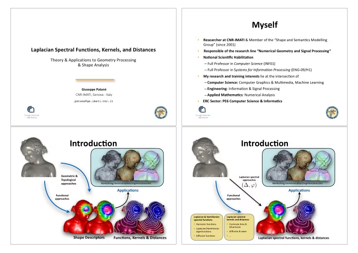
FuncHonal approaches Laplacian spectral approaches

(∆, ϕ)

Main (target) properties

• Intrinsic & multi-scale definition
• Invariance to uniform scaling/isometries
• Generalisation to n-D data
• Easy computation
• Approximation of geodesic & optimal

transportation distances

Laplacian spectral funcHons, kernels & distances

Remeshing/skeletonisa<on/segmenta<on/etc

ApplicaHons

Conclusions

• Review of previous work on

– the Laplacian spectral funcHons, kernels, and distances, defined by filtering the Laplacian spectrum and as a generalisa<on of the commute-<me, bi-harmonic, diffusion, and wave kernel and distances – their discreHsaHon according to a unified representa<on of the Laplace- Beltrami operator, which is “independent” of

• the data dimensionality (surface, volume, nD data) and discre<sa<on

(mesh, point set) of the input domain

• the selected Laplacian weights

– the computaHonal aspects behind their evaluaHon

• approxima<on accuracy & stability
• computa<onal cost & storage overhead
• use of input parameters & heuris<cs

– their main applicaHons to geometry processing and shape analysis

Conclusions

• Future work & possible collaboraHons

– Defini<on of shape-aware funcHons for Hme-varying & mulH- dimensional data (eg., graphs, videos); – Analysis of the constraints on the filter in order to define “op<mal” spectral kernels and distances for applica<ons in geometry processing and shape analysis – Applica<on/specialisa<on of the spectral basis func<ons to

• shape analysis
• definiHon of shape-aware funcHonal spaces where we approximate

signal or solve PDEs

• Course material & Papers

– http://pers.ge.imati.cnr.it/patane/SGP2019/Course.html – http://pers.ge.imati.cnr.it/patane/Home.html

References

An Introduction to Laplacian Spectral Distance and Kernels

Giuseppe Patanè, CNR-IMATI Paperback ISBN: 9781681731391 Ebook ISBN: 9781681731407 Published 07/2017 • 139 pages Paperback: USD $45.95 Ebook: USD $36.76 Combo: USD $57.44

• CONTENTS
• List of Figures
• List of Tables
• Preface
• Acknowledgments
• Laplace-Beltrami Operator
• Heat and Wave Equations
• Laplacian Spectral Distances
• Discrete Spectral Distances
• Applications
• Conclusions
• Bibliography
• Author’s Biography

In geometry processing and shape analysis, several applications have been addressed through the properties of the Laplacian spectral kernels and distances, such as commute-time, biharmonic, difusion, and wave distances. Within this context, this book is intended to provide a common background on the defjnition and computation of the Laplacian spectral kernels and distances for geometry processing and shape analysis. To this end, we defjne a unifjed representation of the isotropic and anisotropic discrete Laplacian operator on surfaces and volumes; then, we introduce the associated diferential equations, i.e., the harmonic equation, the Laplacian eigenproblem, and the heat equation. Filtering the Laplacian spectrum, we introduce the Laplacian spectral distances, which generalize the commute-time, biharmonic, difusion, and wave distances, and their discretization in terms of the Laplacian spectrum. As main applications, we discuss the design of smooth functions and the Laplacian smoothing

• f noisy scalar functions.

All the reviewed numerical schemes are discussed and compared in terms

• f robustness, approximation accuracy, and computational cost, thus

supporting the reader in the selection of the most appropriate with respect to shape representation, computational resources, and target application. ABOUT THE AUTHOR Giuseppe Patane is a researcher at CNR-IMATI (2006-today) Institute for Applied Mathematics and Information Technologies-Italian National Research Council. Since 2001, his research activities have been focused on the defjnition of paradigms and algorithms for modeling and analyzing digital shapes and multidimensional data. He received a Ph.D. in Mathematics and Applications from the University of Genova (2005) .

PRINT & eBOOK at: www.morganclaypoolpublishers.com

1210 Fifth Avenue • Suite 250 • San Rafael, CA 94901

SLIDE 29

Acknowledgments

• People

– SGP2019 Conference & Graduate School Chairs: Marcel Campen & Sylvain Lefebvre – Shape and Seman<cs Modelling Group, CNR-IMATI, Italy

• Projects

– H2020 ERC-AdG CHANGE – IMAGE-FUSION, Biannual Project funded by Regione Liguria & EU FESR

• Shapes

– AIM@SHAPE Repository – SHREC2010/2016 data sets

• Contact: patane@ge.imati.cnr.it