Visualization Visualization Height Fields and Contours Height - PDF document

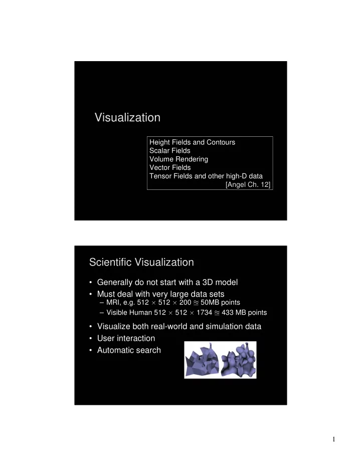
Visualization Visualization Height Fields and Contours Height Fields and Contours Scalar Fields Scalar Fields Volume Rendering Volume Rendering Vector Fields Vector Fields Tensor Fields and other high-D data Tensor Fields and other high-D data [Angel Ch. 12] [Angel Ch. 12] Scientific Visualization Scientific Visualization • Generally do not start with a 3D model • Must deal with very large data sets – MRI, e.g. 512 � 512 � 200 � 50MB points – Visible Human 512 � 512 � 1734 � 433 MB points • Visualize both real-world and simulation data • User interaction • Automatic search 1

Types of Data Types of Data • Scalar fields (3D volume of scalars) – E.g., x-ray densities (MRI, CT scan) • Vector fields (3D volume of vectors) – E.g., velocities in a wind tunnel • Tensor fields (3D volume of tensors [matrices]) – E.g., stresses in a mechanical part [Angel 12.7] • Static or through time Example: Turbulent convection Example: Turbulent convection • Penetrative turbulent convection in a compressible ideal gas (PTCC) • http://www.vets.ucar.edu/vg/PTCC/index.shtml plot of enstrophy (vorticity squared) � 2

Example: Turbulent convection Example: Turbulent convection Example: Turbulent convection Example: Turbulent convection How do we visualize volume data like this? 3

Height Field Height Field • Visualizing an explicit function z = f(x,y) • Adding contour curves g(x,y) = c Meshes Meshes • Function is sampled (given) at x i , y i , 0 � i, j � n • Assume equally spaced • Generate quadrilateral or triangular mesh • [Asst 1] 4

Contour Curves Contour Curves • Recall: implicit curve f(x,y) = 0 • f(x,y) < 0 inside, f(x,y) > 0 outside • Here: contour curve at f(x,y) = c • Sample at regular intervals for x,y • How can we draw the curve? Marching Squares Marching Squares • Sample function f at every grid point x i , y j • For every point f i j = f(x i , y j ) either f i j � c or f i j > c • Distinguish those cases for each corner x – White: f i j � c – Black: f i j > c • Now consider cases for curve • Assume “smooth” • Ignore f i j = 0 5

Interpolating Intersections Interpolating Intersections • Approximate intersection – Midpoint between x i , x i+1 and y j , y j+1 – Better: interpolate • If f i j = a is closer to c than b = f i+1 j then intersection is closer to (x i , y j ): • Analogous calculation x i x i+1 for y direction x f i j = a < c c < b = f i+1 j Cases for Vertex Labels Cases for Vertex Labels 16 cases for vertex labels 4 unique mod. symmetries 6

Ambiguities of Labelings Ambiguities of Labelings Ambiguous labels Different resulting contours Resolution by subdivision (where possible) Marching Squares Examples Marching Squares Examples • Ovals of Cassini, 50 � 50 grid Midpoint Interpolation Contour plot of Honolulu data 7

Outline Outline • Height Fields and Contours • Scalar Fields • Volume Rendering • Vector Fields • Tensor Fields and other high-D data Scalar Fields Scalar Fields • Volumetric data sets • Example: tissue density • Assume again regularly sampled • Represent as voxels 8

Isosurfaces Isosurfaces • f(x,y,z) represents volumetric data set • Two rendering methods – Isosurface rendering – Direct volume rendering (use all values [next]) • Isosurface given by f(x,y,z) = c • Recall implicit surface g(x, y, z): – g(x, y, z) < 0 inside – g(x, y, z) = 0 surface – g(x, y, z) > 0 outside • Generalize right-hand side from 0 to c Marching Cubes Marching Cubes • Display technique for isosurfaces • 3D version of marching squares • 14 cube labelings (after elimination symmetries) 9

Marching Cube Tessellations Marching Cube Tessellations • Generalize marching squares, just more cases • Interpolate as in 2D • Ambiguities similar to 2D Marching Cubes Demo Marching Cubes Demo 10

Volume Rendering Volume Rendering • Sometimes isosurfaces are unnatural • Use all voxels and transparency ( � -values) Volume rendering Ray-traced isosurface Surface vs. Volume Rendering Surface vs. Volume Rendering • 3D model of surfaces • Scalar field in 3D • Convert to triangles • Convert to RGBA values • Draw primitives • Render volume “directly” • Lose or disguise data • See data as given • Good for opaque objects • Good for complex objects 11

Sample Applications Sample Applications • Medical – Computed Tomography (CT) – Magnetic Resonance Imaging (MRI) – Ultrasound • Engineering and Science – Computational Fluid Dynamic (CFD) – Aerodynamic simulations – Meteorology – Astrophysics Volume Rendering Pipeline Volume Rendering Pipeline • Transfer function: from data set to colors and opacities – Example: 256 � 256 � 64 � 2 = 4 MB – Example: use colormap (8 bit color, 8 bit opacity) Transfer function Rendering Data sets Sample Volume Image 12

Transfer Functions Transfer Functions • Transform scalar data values to RGBA values • Apply to every voxel in volume • Highly application dependent • Start from data histogram • Opacity for emphasis Transfer Function Example Transfer Function Example Mantle Convection Scientific Computing and Imaging (SCI) University of Utah 13

Types of Volume Rendering Types of Volume Rendering • Three volume rendering techniques – Volume ray casting – Splatting – 3D texture mapping • Ray Casting – Integrate color and opacity along ray Ray Casting – Accumulating Opacity Ray Casting – Accumulating Opacity • � = 1.0 is opaque • Composite multiple layers according to opacity 14

Real-Time Ray Tracer (Utah) Real-Time Ray Tracer (Utah) Splatting Splatting • Wonderfully simple • Working back-to-front (or front-to-back), draw a “splat” for each chunk of data • Easy to implement, but not as accurate as ray casting • Works reasonably for non-uniform data closeup of a splat 15

Splatting Splatting • Alternative to ray tracing • Assign shape to each voxel (e.g., Gaussian) • Project onto image plane (splat) • Draw voxels back-to-front • Composite ( � -blend) 3D Textures 3D Textures • Alternative to ray tracing, splatting • Build a 3D texture (including opacity) • Draw a stack of polygons, back-to-front • Efficient if supported in graphics hardware • Few polygons, much texture memory 3D RGBA texture Viewpoint Draw back to front 16

Example: 3D Textures Example: 3D Textures Emil Praun’01 Example: 3D Textures Example: 3D Textures Emil Praun’01 17

Other Techniques—CSG is Easy Other Techniques—CSG is Easy • The transfer function can be used to mask a volume or merge volumes • You are still confined to the grid, of course not and head or Outline Outline • Height Fields and Contours • Scalar Fields • Volume Rendering • Vector Fields • Tensor Fields and other high-D data 18

Vector Fields Vector Fields • Visualize vector at each (x,y,z) point – Example: velocity field – Example: hair • Hedgehogs – Use 3D directed line segments (sample field) – Orientation and magnitude determined by vector • Animation – Use for still image – Particle systems Blood flow in human carotid artery Using Glyphs and Streaks Using Glyphs and Streaks Glyphs for air flow University of Utah 19

More Flow Examples More Flow Examples Banks and Interrante Example: Jet Shockwave Example: Jet Shockwave P. Sutton University of Utah http://www.sci.utah.edu/ 20

Visualization in 3D environments Visualization in 3D environments CAVE, Brown Lines can also be used to show shape Lines can also be used to show shape Draw lines in directions of principal curvature Victoria Interrante 21

Interaction: Data Probe Interaction: Data Probe SCI, Utah Outline Outline • Height Fields and Contours • Scalar Fields • Volume Rendering • Vector Fields • Tensor Fields and other high-D data 22

High- High- Dimensional Dimensional Data Data • How do we display data that is very high dimensional? • One idea is to draw inspiration from art David Laidlaw, Brown 23

24

Summary Summary • Height Fields and Contours • Scalar Fields – Isosurfaces – Marching cubes • Volume Rendering – Volume ray tracing – Splatting – 3D Textures • Vector Fields – Hedgehogs – Animated and interactive visualization • Tensor Fields and other High-Dimensional Data – NPR and other art-motivated techniques 25

Top Visualization Research Issues • Error and Uncertainty Visual Representation • Perceptual Issues • Quantify Effectiveness • Time Dependent Visualization • Pipeline Complexity • Think About the Science • Interesting Feature Detection • Leverage both Hardware and Software Methods • Multi-field Visualization From Chris Johnson, Utah 26