Variational principle (Ch. 7) Only Sec. 7.1 Theorem: For an - - PowerPoint PPT Presentation

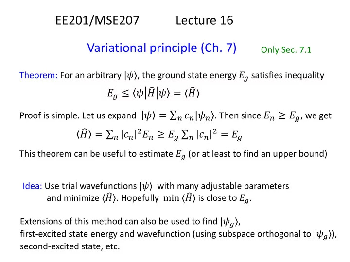
Variational principle (Ch. 7)

Only Sec. 7.1 Theorem: For an arbitrary |𝜔〉, the ground state energy 𝐹𝑕 satisfies inequality

𝐹𝑕 ≤ 𝜔 𝐼 𝜔 = 〈 𝐼〉

Proof is simple. Let us expand 𝜔 = 𝑜 𝑑𝑜|𝜔𝑜〉. Then since 𝐹𝑜 ≥ 𝐹𝑕, we get

𝐼 = 𝑜 𝑑𝑜 2𝐹𝑜 ≥ 𝐹𝑕 𝑜 𝑑𝑜 2 = 𝐹𝑕

This theorem can be useful to estimate 𝐹𝑕 (or at least to find an upper bound) Idea: Use trial wavefunctions |𝜔〉 with many adjustable parameters and minimize 〈 𝐼〉. Hopefully min 〈 𝐼〉 is close to 𝐹𝑕. Extensions of this method can also be used to find |𝜔𝑕〉, first-excited state energy and wavefunction (using subspace orthogonal to |𝜔𝑕〉), second-excited state, etc.

EE201/MSE207 Lecture 16

EE201/MSE207 Lecture 16

Band structure (back to Ch. 5)

Band structure for electrons is a consequence of a periodic potential in a lattice (due to periodic arrangement of atoms). Bloch’s theorem: If 𝑊 𝑦 + 𝑏 = 𝑊(𝑏), then for an eigenstate of energy Proof

𝜔(𝑦 + 𝑏) = 𝑓𝑗𝐿𝑏 𝜔 𝑦

(almost periodic, “quasimomentum” ℏ𝐿) It commutes with Hamiltonian, 𝐸, 𝐼 = 0, therefore common eigenfunctions. If 𝜇 ≠ 1, then 𝜔 would increase or decrease exponentially Introduce displacement operator 𝐸, so that 𝐸𝑔(𝑦) = 𝑔(𝑦 + 𝑏). For simplicity let us consider 1D case

𝑊 𝑦 + 𝑏 = 𝑊(𝑦)

(periodic with lattice constant 𝑏)

𝜔 𝑦 + 𝑏 = 𝜇 𝜔 𝑦

Therefore 𝜇 = 1, can denote 𝜇 = 𝑓𝑗𝐿𝑏. Therefore 𝜔 𝑦 = 𝑓𝑗𝐿𝑦

𝜔(𝑦) with periodic

𝜔(𝑦),

𝜔 𝑦 + 𝑏 = 𝜔(𝑦)

Periodic boundary condition for Bloch’s theorem

Then

𝜔 𝑦 + 𝑂𝑏 = 𝜔(𝑦)

Usually people use periodic boundary condition in using Bloch’s theorem

𝑊 𝑦 + 𝑏 = 𝑊 𝑏

⇒

𝜔(𝑦 + 𝑏) = 𝑓𝑗𝐿𝑏 𝜔 𝑦

for 𝑂 ⋙ 1 atoms in a (1D) sample Why? Because it does not matter, but makes calculations simpler

𝐿 = 2𝜌𝑜 𝑂𝑏 , 𝑜 = 0, ±1, ±2, …

This gives 𝑂 different values of 𝐿 (the same 𝑓𝑗𝐿𝑏 if Δ𝑜 = 𝑂): 𝑂 states in a band for 𝑂 atoms Since 𝑂 is very large, 𝐿 is almost continuous.

Simple example: “Dirac comb”

Dirac comb: 0 < 𝑦 < 𝑏 ⇒ 𝜔 𝑦 = 𝐵 sin(𝑙𝑦) + 𝐶 cos 𝑙𝑦 ,

𝑙 = 2𝑛𝐹/ℏ 𝑊 𝑦 = 𝛽 𝑘=1

𝑂

𝜀(𝑦 − 𝑘𝑏)

(wrapped around)

− ℏ2 2𝑛 𝑒2𝜔 𝑦 𝑒𝑦2 + 𝑊 𝑦 𝜔 𝑦 = 𝐹 𝜔 𝑦

From Bloch’s theorem we know that at −𝑏 < 𝑦 < 0, 𝜔 𝑦 = 𝑓−𝑗𝐿𝑏[𝐵 sin 𝑙(𝑦 + 𝑏) + 𝐶 cos 𝑙(𝑦 + 𝑏) ]

𝜔 0 + 0 = 𝜔 0 − 0 ⇒ 𝐶 = 𝑓−𝑗𝐿𝑏 [𝐵 sin 𝑙𝑏 + 𝐶 cos(𝑙𝑏)] 𝜔′ 0 + 0 − 𝜔′ 0 − 0 = ( 2𝑛𝛽 ℏ2) 𝜔(0) ⇒ 𝑙𝐵 − 𝑓−𝑗𝐿𝑏[𝑙𝐵 cos 𝑙𝑏 − 𝑙𝐶 sin(𝑙𝑏) ] = ( 2𝑛𝛽 ℏ2) 𝐶

From these two equations we find (eliminating 𝐵 and 𝐶)

cos 𝐿𝑏 = cos 𝑙𝑏 + 𝑛𝛽𝑏 ℏ2 sin(𝑙𝑏) 𝑙𝑏

𝑂 “atoms”

Dirac comb (cont.)

𝑊 𝑦 = 𝛽 𝑘=1

𝑂

𝜀(𝑦 − 𝑘𝑏)

cos 𝐿𝑏 = cos 𝑙𝑏 + 𝑛𝛽𝑏 ℏ2 sin(𝑙𝑏) 𝑙𝑏

𝑛𝛽𝑏 ℏ2 = 10 𝑙𝑏 (∝ 𝐹) 𝐿𝑏 = 2𝜌𝑜 𝑂 𝑂 states

1st band 2nd band 3rd band

gap gap gap 𝑂 states 𝑂 states 𝑂 states 𝑂 states per band (× 2 spin) gap gap Gaps become smaller, eventually continuum

Bands

𝑂 states per band (× 2 spin) Gaps become smaller, eventually continuum If one electron per atom (𝑟 = 1), then half a band is filled (good conductor) If 𝑟 = 2, then one band is filled completely (insulator

• r semiconductor; cannot slightly excite electrons)

If 𝑟 = 3, then 1.5 bands are filled (good conductor) Metals usually have 𝑟 = 1 If 𝑟 = 4, then again insulator or semiconductor Etc.

Bands (cont.)

ℏ𝐿 is quasimomentum

(behaves as momentum)

𝐹 = ℏ2𝑙2 2𝑛

For a free particle

∝ 𝐹

𝜌/𝑏 −𝜌/𝑏 2𝜌/𝑏 2𝜌/𝑏

(Brillouin zone)

Define effective mass 𝑛eff via Δ𝐹 = ℏ2𝐿2

2𝑛eff

• r even

Δ𝐹 = ℏ2(Δ𝐿)2 2𝑛eff

• r even

𝑒2𝐹 𝑒𝐿2 = ℏ2 𝑛eff

(similar to bands in semiconductors)

Periodic:

cos 𝐿𝑏 = . . .

Quasimomentum ℏ𝐿 behaves as momentum

Let us add small force 𝐺 (e.g., due to electric field acting on electron, 𝐺 = −𝑓ℰ ). From Bloch’s theorem we know 𝜔 𝑦 = 𝑓𝑗𝐿𝑦 𝜔𝐿(𝑦) ∝ 𝑓𝑗𝐿𝑦 on the large scale It means

Ψ 𝑦, 𝑢 ∝ 𝑓𝑗𝐿𝑦𝑓−𝑗 𝐹−𝐺𝑦 𝑢

ℏ

= 𝑓𝑗 𝐿+ 𝐺𝑢

ℏ 𝑦 𝑓−𝑗𝐹𝑢/ℏ

We see that ℏ𝐿 behaves as momentum (so named quasimomentum)

𝐿 → 𝐿 + 𝐺 ℏ 𝑢 ⇒

(for validity of this approach we need very small 𝐺) Then Δ𝑊 = −𝐺𝑦 and therefore 𝐹 → 𝐹 − 𝐺𝑦 (for the same 𝐿). Adding time dependence, we get (on the large scale) Actually, significant oversimplification in this approach; this rather a hint. More rigorously,

𝑓𝑗(𝐿+

𝐺𝑢 ℏ)𝑦𝑓 − 𝑗 ℏ

𝑢 𝐹(𝐿+𝐺

𝑢′ ℏ) 𝑒𝑢′

𝜔𝐿+𝐺

𝑢 ℏ(𝑦)

is an approximate solution of SE (straightforward to check).

𝑒(ℏ𝐿) 𝑒𝑢 = 𝐺

Also, makes sense for energy change: 𝐺𝑤𝑕𝑠 = ℏ 𝑒𝐿

𝑒𝑢 𝑒𝐹 ℏ 𝑒𝐿 = 𝑒𝐹 𝑒𝑢 .

End of material included into the final exam

Following lectures are important, but not needed for the exam