Appendix: Appendix: Other ATPG algorithms Other ATPG algorithms 1 - - PDF document

▶

Mar 21, 2023 453 likes •602 views

4/28/2009 Appendix: Appendix: Other ATPG algorithms Other ATPG algorithms 1 TOPS Dominators TOPS Dominators Kirkland and Mercer (1987) Kirkland and Mercer (1987) Dominator of g all paths from g to PO must pass through the

SLIDE 1

4/28/2009 1

Appendix: Other ATPG algorithms Appendix: Other ATPG algorithms

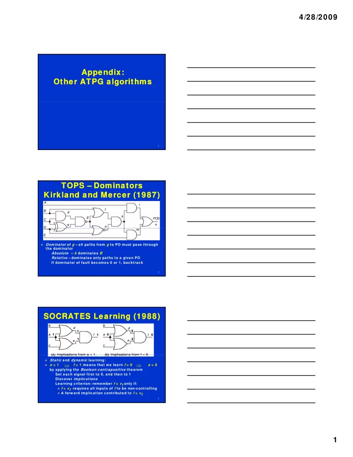
TOPS – Dominators Kirkland and Mercer (1987) TOPS – Dominators Kirkland and Mercer (1987)

 Dominator of g – all paths from g to PO must pass through

the dominator Absolute -- k dominates B Relative – dominates only paths to a given PO If dominator of fault becomes 0 or 1, backtrack

SOCRATES Learning (1988) SOCRATES Learning (1988)

 Static and dynamic learning:  a = 1 f = 1 means that w e learn f = 0 a = 0

by applying the Boolean contrapositive theorem Set each signal first to 0, and then to 1 Discover implications Learning criterion: remember f = vf only if:

 f = vf requires all inputs of f to be non-controlling  A forw ard implication contributed to f = vf

 

SLIDE 2

4/28/2009 2

Improved Unique Sensitization Procedure Improved Unique Sensitization Procedure

 When a is only D-frontier signal, find dominators

f a and set their inputs unreachable from a to 1

 Find dominators of single D-frontier signal a and

make common input signals non-controlling

Constructive Dilemma Constructive Dilemma

 [(a = 0) (i = 0)] [(a = 1) (i = 0)] (i = 0)  If both assignments 0 and 1 to a make i = 0,

then i = 0 is implied independently of a

   

Modus Tollens and Dynamic Dominators Modus Tollens and Dynamic Dominators

 Modus Tollens:

(f = 1) [(a = 0) (f = 0)] (a = 1)

  

 Dynamic dominators:

Compute dominators and dynamically learned implications after each decision step Too computationally expensive

SLIDE 3

4/28/2009 3

EST – Dynamic Programming (Giraldi & Bushnell) EST – Dynamic Programming (Giraldi & Bushnell)

 E-frontier – partial circuit functional decomposition

Equivalent to a node in a BDD Cut-set betw een circuit part w ith know n labels and part w ith X signal labels

 EST learns E-frontiers during ATPG and stores them in

a hash table a hash table Dynamic programming – w hen new decomposition generated from implications of a variable assignment, looks it up in the hash table Avoids repeating a search already conducted

 Terminates search w hen decomposition matches:

Earlier one that lead to a test (retrieves stored test) Earlier one that lead to a backtrack

 Accelerated SOCRATES nearly 5.6 times 7

Fault B sa1 Fault B sa1

Fault h sa1 Fault h sa1

SLIDE 4

4/28/2009 4

Implication Graph ATPG Chakradhar et al. (1990) Implication Graph ATPG Chakradhar et al. (1990)

 Model logic behavior using implication graphs

Nodes for each literal and its complement Arc from literal a to literal b means that if a = 1 then b must also be 1

 Extended to find implications by using a graph

transitive closure algorithm – finds paths of edges Made much better decisions than earlier ATPG search algorithms Uses a topological graph sort to determine

rder of setting circuit variables during ATPG

Example and Implication Graph Example and Implication Graph

Graph Transitive Closure Graph Transitive Closure

 When d set to 0, add edge from d to d,

w hich means that if d is 1, there is conflict w hich means that if d is 1, there is conflict Can deduce that (a = 1) F

 When d set to 1, add edge from d to d



SLIDE 5

4/28/2009 5

Consequence of F = 1 Consequence of F = 1

 Boolean false function F (inputs d and e) has deF  For F = 1, add edge F F so deF reduces to d e  To cause de = 0 w e add edges: e d and d e

Now , w e find a path in the graph b b So b cannot be 0, or there is a conflict

 Therefore b = 1 is a consequence of F = 1

   

 Therefore, b = 1 is a consequence of F = 1

Related Contributions Related Contributions

 Larrabee – NEMESIS -- Test generation using

satisfiability and implication graphs

 Chakradhar, Bushnell, and Agraw al – NNATPG –

ATPG using neural netw orks & implication graphs

 Chakradhar, Agraw al, and Rothw eiler – TRAN --

T iti Cl t t ti l ith Transitive Closure test generation algorithm

 Cooper and Bushnell – Sw itch-level ATPG  Agraw al, Bushnell, and Lin – Redundancy

identification using transitive closure

 Stephan et al. – TEGUS – satisfiability ATPG  Henftling et al. and Tafertshofer et al. – ANDing

node in implication graphs for efficient solution

Recursive Learning Kunz and Pradhan (1992) Recursive Learning Kunz and Pradhan (1992)

 Applied SOCRATES type learning

recursively Maximum recursion depth r Maximum recursion depth rmax determines w hat is learned about circuit Time complexity exponential in rmax Memory grow s linearly w ith rmax

SLIDE 6

4/28/2009 6

Recursive_Learning Algorithm Recursive_Learning Algorithm

for each unjustified line for each input: justification assign controlling value; make implications and set up new list of unjustified lines; if (consistent) Recursive_Learning (); if (> 0 signals f w ith same value V for all consistent justifications) learn f = V; make implications for all learned values; if (all justifications inconsistent) learn current value assignments as consistent;

Recursive Learning Recursive Learning

 i1 = 0 and j = 1 unjustifiable – enter learning

i1 = 0 a1 b1 c1 d1 b a d c f1 e1 g1 j = 1 h k d1 d d2 c2 b2 a2 f2 e2 h2 g2 h1 i2

Justify i1 = 0 Justify i1 = 0

 Choose first of 2 possible assignments g1 = 0

i1 = 0 a1 b1 c1 d1 b a d c f1 e1 g1 = 0 j = 1 h k d1 d d2 c2 b2 a2 f2 e2 h2 g2 h1 i2

SLIDE 7

4/28/2009 7

Implies e1 = 0 and f1 = 0 Implies e1 = 0 and f1 = 0

 Given that g1 = 0

i1 = 0 a1 b1 c1 d1 b a d c g1 = 0 f1 = 0 e1 = 0 j = 1 h k d1 d d2 c2 b2 a2 f2 e2 h2 g2 h1 i2 f1 = 0

Justify a1 = 0, 1st Possibility Justify a1 = 0, 1st Possibility

 Given that g1 = 0, one of tw o possibilities

i1 = 0 a1 = 0 b1 c1 d1 b a d c g1 = 0 f1 = 0 e1 = 0 j = 1 h k d1 d d2 c2 b2 a2 f2 e2 h2 g2 h1 i2 f1 = 0

Implies a2 = 0 Implies a2 = 0

 Given that g1 = 0 and a1 = 0

i1 = 0 a1 = 0 b1 c1 d1 b a d c g1 = 0 f1 = 0 e1 = 0 j = 1 h k d1 d d2 c2 b2 a2 = 0 f2 e2 h2 g2 h1 i2 f1 = 0

SLIDE 8

4/28/2009 8

Implies e2 = 0 Implies e2 = 0

 Given that g1 = 0 and a1 = 0

i1 = 0 a1 = 0 b1 c1 d1 b a d c g1 = 0 f1 = 0 e1 = 0 j = 1 h k d1 d d2 c2 b2 a2 = 0 f2 e2 = 0 h2 g2 h1 i2 f1 = 0

Now Try b1 = 0, 2 nd Option Now Try b1 = 0, 2 nd Option

 Given that g1 = 0

i1 = 0 a1 b1 = 0 c1 d1 b a d c g1 = 0 f1 = 0 e1 = 0 j = 1 h k d1 d d2 c2 b2 a2 f2 e2 h2 g2 h1 i2 f1 = 0

Implies b2 = 0 and e2 = 0 Implies b2 = 0 and e2 = 0

 Given that g1 = 0 and b1 = 0

i1 = 0 a1 b1 = 0 c1 d1 b a d c g1 = 0 f1 = 0 e1 = 0 j = 1 h k d1 d d2 c2 b2 = 0 a2 f2 e2 = 0 h2 g2 h1 i2 f1 = 0

SLIDE 9

4/28/2009 9

Both Cases Give e2 = 0, So Learn That Both Cases Give e2 = 0, So Learn That

i1 = 0 a1 b1 c1 d1 b a d c g1 = 0 f1 = 0 e1 = 0 j = 1 h k d1 d d2 c2 b2 a2 f2 e2 = 0 h2 g2 h1 i2 f1 = 0

Justify f1 = 0 Justify f1 = 0

 Try c1 = 0, one of tw o possible assignments

i1 = 0 a1 b1 c1 = 0 d1 b a d c g1 = 0 f1 = 0 e1 = 0 j = 1 h k d1 d d2 c2 b2 a2 f2 e2 = 0 h2 g2 h1 i2 f1 = 0

Implies c2 = 0 Implies c2 = 0

 Given that c1 = 0, one of tw o possibilities

i1 = 0 a1 b1 c1 = 0 d1 b a d c g1 = 0 f1 = 0 e1 = 0 j = 1 h k d1 d d2 c2 = 0 b2 a2 f2 e2 = 0 h2 g2 h1 i2 f1 = 0

SLIDE 10

4/28/2009 10

Implies f2 = 0 Implies f2 = 0

 Given that c1 = 0 and g1 = 0

i1 = 0 a1 b1 c1 = 0 d1 b a d c g1 = 0 f1 = 0 e1 = 0 j = 1 h k d1 d d2 c2 = 0 b2 a2 f2 = 0 e2 = 0 h2 g2 h1 i2 f1 = 0

Try d1 = 0 Try d1 = 0

 Try d1 = 0, second of tw o possibilities

i1 = 0 a1 b1 c1 d1 = 0 b a d c g1 = 0 f1 = 0 e1 = 0 j = 1 h k d1 = 0 d d2 c2 b2 a2 f2 e2 = 0 h2 g2 h1 i2 f1 = 0

Implies d2 = 0 Implies d2 = 0

 Given that d1 = 0 and g1 = 0

i1 = 0 a1 b1 c1 d1 = 0 b a d c g1 = 0 f1 = 0 e1 = 0 j = 1 h k d1 = 0 d d2 = 0 c2 b2 a2 f2 e2 = 0 h2 g2 h1 i2 f1 = 0

SLIDE 11

4/28/2009 11

Implies f2 = 0 Implies f2 = 0

 Given that d1 = 0 and g1 = 0

i1 = 0 a1 b1 c1 d1 = 0 b a d c g1 = 0 f1 = 0 e1 = 0 j = 1 h k d1 = 0 d d2 = 0 c2 b2 a2 f2 = 0 e2 = 0 h2 g2 h1 i2 f1 = 0

Since f2 = 0 In Either Case, Learn f2 = 0 Since f2 = 0 In Either Case, Learn f2 = 0

i1 = 0 a1 b1 c1 d1 b a d c g1 = 0 f1 e1 j = 1 h k d1 d d2 c2 b2 a2 f2 = 0 e2 = 0 h2 g2 h1 i2 f1

Implies g2 = 0 Implies g2 = 0

i1 = 0 a1 b1 c1 d1 b a d c g1 = 0 f1 e1 j = 1 h k d1 d d2 c2 b2 a2 f2 = 0 e2 = 0 h2 g2 = 0 h1 i2 f1

SLIDE 12

4/28/2009 12

Implies i2 = 0 and k = 1 Implies i2 = 0 and k = 1

i1 = 0 a1 b1 c1 d1 b a d c g1 = 0 f1 e1 j = 1 h k = 1 d1 d d2 c2 b2 a2 f2 = 0 e2 = 0 h2 g2 = 0 h1 i2 = 0 f1

Justify h1 = 0 Justify h1 = 0

i1 = 0 a1 b1 c1 d1 b a d c f1 e1 g1

Second of two possibilities to make i1 = 0

j = 1 h k d1 d d2 c2 b2 a2 f2 e2 h2 g2 h1 = 0 i2

Implies h2 = 0 Implies h2 = 0

 Given that h1 = 0

i1 = 0 a1 b1 c1 d1 b a d c f1 e1 g1 j = 1 h k d1 d d2 c2 b2 a2 f2 e2 h2 = 0 g2 h1 = 0 i2

SLIDE 13

4/28/2009 13

Implies i2 = 0 and k = 1 Implies i2 = 0 and k = 1

 Given 2 nd of 2 possible assignments h1 = 0

i1 = 0 a1 b1 c1 d1 b a d c f1 e1 g1 j = 1 h k = 1 d1 d d2 c2 b2 a2 f2 e2 h2 = 0 g2 h1 = 0 i2 = 0

Both Cases Cause k = 1 (Given j = 1), i2 = 0 Both Cases Cause k = 1 (Given j = 1), i2 = 0

 Therefore, learn both independently

i1 = 0 a1 b1 c1 d1 b a d c f1 e1 g1 j = 1 h k = 1 d1 d d2 c2 b2 a2 f2 e2 h2 g2 h1 i2 = 0

Other ATPG Algorithms Other ATPG Algorithms

 Legal assignment ATPG (Rajski and Cox)

Maintains pow er-set of possible assignments on each node {0, 1, D, D, X}

 BDD-based algorithms

Catapult (Gaede, Mercer, Butler, Ross) p ( , , , ) Tsunami (Stanion and Bhattacharya) – maintains BDD fragment along fault propagation path and incrementally extends it Unable to do highly reconverging circuits (parallel multipliers) because BDD essentially becomes infinite