The Structure of Hidden Markov Models Have N states, states 1 . . . - - PowerPoint PPT Presentation

6.864 (Fall 07) The EM Algorithm Part II

1

Overview

• Hidden Markov models
• The EM algorithm in general form
• Products of multinomial (PM) models
• The EM algorithm for PM models
• The EM algorithm for hidden markov models (dynamic

programming)

2

The Structure of Hidden Markov Models

• Have N states, states 1 . . . N
• Without loss of generality, take N to be the final or stop state
• Have an alphabet Σ. For example Σ = {a, b}
• Parameter πi for i = 1 . . . N is probability of starting in state i
• Parameter ai,j for i = 1 . . . (N − 1), and j = 1 . . . N is

probability of state j following state i

• Parameter bi(o) for i = 1 . . . (N −1), and o ∈ Σ is probability
• f state i emitting symbol o

3

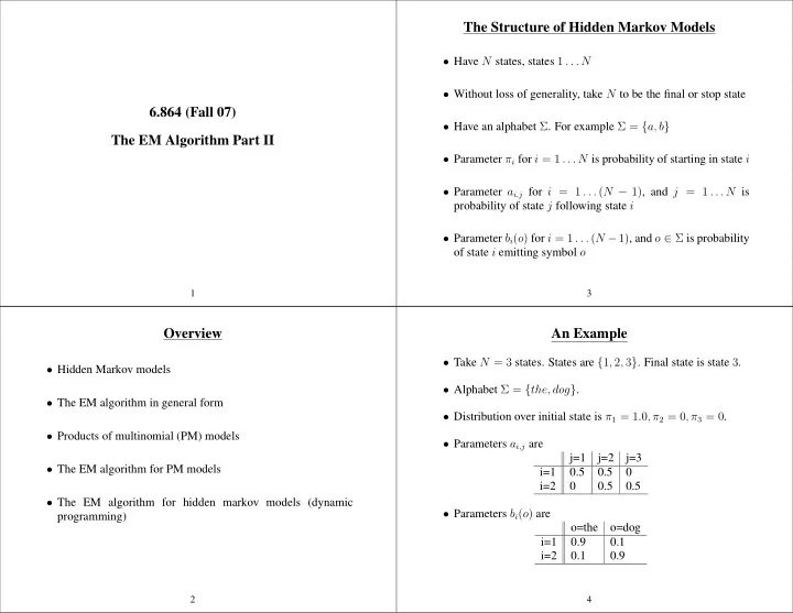
An Example

• Take N = 3 states. States are {1, 2, 3}. Final state is state 3.
• Alphabet Σ = {the, dog}.
• Distribution over initial state is π1 = 1.0, π2 = 0, π3 = 0.
• Parameters ai,j are

j=1 j=2 j=3 i=1 0.5 0.5 i=2 0.5 0.5

• Parameters bi(o) are
• =the
• =dog

i=1 0.9 0.1 i=2 0.1 0.9

4

A Generative Process

• Pick the start state s1 to be state i for i = 1 . . . N with

probability πi.

• Set t = 1
• Repeat while current state st is not the stop state (N):

– Emit a symbol ot ∈ Σ with probability bst(ot) – Pick the next state st+1 as state j with probability ast,j. – t = t + 1

5

Probabilities Over Sequences

• An output sequence is a sequence of observations o1 . . . oT

where each oi ∈ Σ e.g. the dog the dog dog the

• A state sequence is a sequence of states s1 . . . sT where each

si ∈ {1 . . . N} e.g. 1 2 1 2 2 1

• HMM defines a probability for each state/output sequence pair

e.g. the/1 dog/2 the/1 dog/2 the/2 dog/1 has probability π1 b1(the) a1,2 b2(dog) a2,1 b1(the) a1,2 b2(dog) a2,2 b2(the) a2,1 b1(dog)a1,3

6

Hidden Markov Models

• An HMM specifies a probability for each possible (x, y) pair,

where x is a sequence of symbols drawn from Σ, and y is a sequence of states drawn from the integers 1 . . . (N − 1). The sequences x and y are restricted to have the same length.

• E.g., say we have an HMM with N = 3, Σ = {a, b}, and with

some choice of the parameters Θ. Take x = a, a, b, b and y = 1, 2, 2, 1. Then in this case, P(x, y|Θ) = π1 a1,2 a2,2 a2,1 a1,3 b1(a) b2(a) b2(b) b1(b)

7

Hidden Markov Models

In general, if we have the sequence x = x1, x2, . . . xn where each xj ∈ Σ, and the sequence y = y1, y2, . . . yn where each yj ∈ 1 . . . (N − 1), then P(x, y|Θ) = πy1ayn,N

n

• j=2

ayj−1,yj

n

• j=1

byj(xj)

8

A Hidden Variable Problem

• We have an HMM with N = 3, Σ = {e, f, g, h}
• We see the following output sequences in training data

e g e h f h f g

• How would you choose the parameter values for πi, ai,j, and

bi(o)?

9

Another Hidden Variable Problem

• We have an HMM with N = 3, Σ = {e, f, g, h}
• We see the following output sequences in training data

e g h e h f h g f g g e h

• How would you choose the parameter values for πi, ai,j, and

bi(o)?

10

Overview

• Hidden Markov models
• The EM algorithm in general form
• Products of multinomial (PM) models
• The EM algorithm for PM models
• The EM algorithm for hidden markov models (dynamic

programming)

11

EM: the Basic Set-up

• We have some data points—a “sample”—x1, x2, . . . xm.
• For example, each xi might be a sentence such as “the

dog slept”: this will be the case in EM applied to hidden Markov models (HMMs) or probabilistic context-free- grammars (PCFGs). (Note that in this case each xi is a sequence, which we will sometimes write xi

1, xi 2, . . . xi ni where

ni is the length of the sequence.)

• Or in the three coins example (see the lecture notes), each xi

might be a sequence of three coin tosses, such as HHH, THT,

• r TTT.

12

• We have a parameter vector Θ.

For example, see the description of HMMs in the previous section. As another example, in a PCFG, Θ would contain the probability P(α → β|α) for every rule expansion α → β in the context-free grammar within the PCFG.

13

• We have a model P(x, y|Θ): A function that for any x, y, Θ

triple returns a probability, which is the probability of seeing x and y together given parameter settings Θ.

• This model defines a joint distribution over x and y, but that we

can also derive a marginal distribution over x alone, defined as P(x|Θ) =

• y

P(x, y|Θ)

14

• Given the sample x1, x2, . . . xm, we define the likelihood as

L′(Θ) =

m

• i=1

P(xi|Θ) =

m

• i=1
• y

P(xi, y|Θ) and we define the log-likelihood as L(Θ) = log L′(Θ) =

m

• i=1

log P(xi|Θ) =

m

• i=1

log

• y

P(xi, y|Θ)

15

• The maximum-likelihood estimation problem is to find

ΘML = arg max

Θ∈Ω L(Θ)

where Ω is a parameter space specifying the set of allowable parameter settings. In the HMM example, Ω would enforce the restrictions N

j=1 πj = 1, for all j = 1 . . . (N − 1),

N

k=1 aj,k = 1, and for all j = 1 . . . (N − 1),

• ∈Σ bj(o) = 1.

16

The EM Algorithm

• Θt is the parameter vector at t’th iteration
• Choose Θ0 (at random, or using various heuristics)
• Iterative procedure is defined as

Θt = argmaxΘQ(Θ, Θt−1) where Q(Θ, Θt−1) =

• i
• y∈Y

P(y | xi, Θt−1) log P(xi, y | Θ)

17

The EM Algorithm

• Iterative procedure is defi ned as Θ

t = argmaxΘQ(Θ, Θt−1), where

Q(Θ, Θt−1) =

• i
• y∈Y

P(y | xi, Θt−1) log P(xi, y | Θ)

• Key points:

– Intuition: fi ll in hidden variables y according to P(y | x

i, Θ)

– EM is guaranteed to converge to a local maximum, or saddle-point,

• f the likelihood function

– In general, if argmaxΘ

• i

log P(xi, yi | Θ) has a simple (analytic) solution, then argmaxΘ

• i
• y

P(y | xi, Θt−1) log P(xi, y | Θ) also has a simple (analytic) solution. 18

Overview

• Hidden Markov models
• The EM algorithm in general form
• Products of multinomial (PM) models
• The EM algorithm for PM models
• The EM algorithm for hidden markov models (dynamic

programming)

19

Products of Multinomial (PM) Models

• In a PCFG, each sample point x is a sentence, and each y is a

possible parse tree for that sentence. We have P(x, y|Θ) =

n

• i=1

P(αi → βi|αi) assuming that (x, y) contains the n context-free rules αi → βi for i = 1 . . . n.

• For example,

if (x, y) contains the rules S → NP VP, NP → Jim, and VP → sleeps, then P(x, y|Θ) = P(S → NP VP|S)×P(NP → Jim|NP)×P(VP → sleeps|VP)

20

Products of Multinomial (PM) Models

• HMMs define a model with a similar form.

Recall the example in the section on HMMs, where we had the following probability for a particular (x, y) pair: P(x, y|Θ) = π1 a1,2 a2,2 a2,1 a1,3 b1(a) b2(a) b2(b) b1(b)

21

Products of Multinomial (PM) Models

• In both HMMs and PCFGs, the model can be written in the

following form P(x, y|Θ) =

• r=1...|Θ|

ΘCount(x,y,r)

r

Here: – Θr for r = 1 . . . |Θ| is the r’th parameter in the model – Count(x, y, r) for r = 1 . . . |Θ| is a count corresponding to how many times Θr is seen in the expression for P(x, y|Θ).

• We will refer to any model that can be written in this form as

a product of multinomials (PM) model.

22

Overview

• Hidden Markov models
• The EM algorithm in general form
• Products of multinomial (PM) models
• The EM algorithm for PM models
• The EM algorithm for hidden markov models (dynamic

programming)

23

The EM Algorithm for PM Models

• We will use Θt to denote the parameter values at the t’th

iteration of the algorithm.

• In the initialization step, some choice for initial parameter

settings Θ0 is made.

• The algorithm then defines an iterative sequence of parameters

Θ0, Θ1, . . . , ΘT, before returning ΘT as the final parameter settings.

• Crucial detail: deriving Θt from Θt−1

24

The EM Algorithm for PM Models: Step 1

• At each iteration of the algorithm, two steps are taken.
• Step 1: expected counts Count(r) are calculated for each

parameter Θr in the model. Count(r) =

m

• i=1
• y

P(y|xi, Θt−1)Count(xi, y, r)

25

The EM Algorithm for PM Models: Step 1

• For example, say we are estimating the parameters of a PCFG

using the EM algorithm. Take a particular rule, such as S → NP V P. Then at the t’th iteration,

Count(S → NP V P) =

m

• i=1
• y

P(y|xi, Θt−1)Count(xi, y, S → NP V P) 26

The EM Algorithm for PM Models: Step 2

• Step 2: Calculate the updated parameters Θt. For example,

we would re-estimate P(S → NP V P|S) = Count(S → NP V P)

• S→β∈R Count(S → β)

Note that the denominator in this term involves a summation

• ver all rules of the form S → β in the grammar. This term

ensures that

• S→β∈R P(S → β|S) = 1, the usual constraint
• n rule probabilities in PCFGs.

27

The EM Algorithm for HMMs: Step 1

• Define Count(xi, y, p → q) to be the number of times a

transition from state p to state q is seen in y.

• Step 1: Calculate expected counts such as

Count(1 → 2) =

m

• i=1
• y

P(y|xi, Θt−1)Count(xi, y, 1 → 2)

• (Note: similar counts will be calculated for emission and

initial-state parameters)

28

The EM Algorithm for HMMs: Step 2

• Step 2: Re-estimate transition parameter as

a1,2 = Count(1 → 2)

N

k=1 Count(1 → k)

where in this case the denominator ensures that N

k=1 a1,k = 1.

• Similar calculations will be performed for other transition

parameters, as well as the initial state parameters and emission parameters.

29

Inputs: A sample of m points, x1, x2, . . . , xm. A model P(x, y|Θ) which takes the following form: P(x, y|Θ) =

• r=1...|Θ|

ΘCount(x,y,r)

r

Initialization: Choose some initial value for the parameters, call this Θ0. Algorithm: For t = 1 . . . T,

• For r = 1 . . . |Θ|, set Count(r) = 0
• For i = 1 . . . m,

– For all y, calculate ty = P(xi, y|Θt−1) – Set sum =

y ty

– For all y, set uy = ty/sum (note that uy = P(y|xi, Θt−1)) – For all r = 1 . . . |Θ|, set Count(r) = Count(r) +

y uyCount(xi, y, r)

• For all r = 1 . . . |Θ|, set

Θt

r = Count(r)

Z where Z is a normalization constant that ensures that the multinomial distribution

• f which Θt

r is a member sums to 1.

Output: Return parameter values ΘT

30

Overview

• Hidden Markov models
• The EM algorithm in general form
• Products of multinomial (PM) models
• The EM algorithm for PM models
• The EM algorithm for hidden markov models (dynamic

programming)

31

The Forward-Backward Algorithm for HMMs

• Define Count(xi, y, p → q) to be the number of times a

transition from state p to state q is seen in y.

• Step 1: Calculate expected counts such as

Count(1 → 2) =

m

• i=1
• y

P(y|xi, Θt−1)Count(xi, y, 1 → 2)

• A problem: the inner sum
• y

P(y|xi, Θt−1)Count(xi, y, 1 → 2)

32

The Forward-Backward Algorithm for HMMs

• Fortunately, there is a way of avoiding this brute force strategy

with HMMs, using a dynamic programming algorithm called the forward-backward algorithm.

• Say that we could efficiently calculate the following quantities

for any x of length n, for any j ∈ 1 . . . n, and for any p ∈ 1 . . . (N − 1) and q ∈ 1 . . . N: P(yj = p, yj+1 = q|x, Θ) =

• y:yj=p,yj+1=q

P(y|x, Θ)

• The inner sum can now be re-written using terms such as this:
• y

P(y|xi, Θt−1)Count(xi, y, p → q) =

ni

• j=1

P(yj = p, yj+1 = q|xi, Θt−1)

33

The Forward Probabilities

Given an input sequence x1 . . . xn, we will define the forward probabilities as being αp(j) = P(x1 . . . xj−1, yj = p | Θ) for all j ∈ 1 . . . n, for all p ∈ 1 . . . N − 1.

34

The Forward Probabilities

Given an input sequence x1 . . . xn, we will define the backward probabilities as being βp(j) = P(xj . . . xn | yj = p, Θ) for all j ∈ 1 . . . n, for all p ∈ 1 . . . N − 1.

35

Given the forward and backward probabilities, the first thing we can calculate is the following: Z = P(x1, x2, . . . xn|Θ) =

• p

αp(j)βp(j) for any j ∈ 1 . . . n. Thus we can calculate the probability of the sequence x1, x2, . . . xn being emitted by the HMM.

36

We can calculate the probability of being in any state at any position: P(yj = p|x, Θ) = αp(j)βp(j) Z for any p, j.

37

We can calculate the probability of each possible state transition, as follows: P(yj = p, yj+1 = q|x, Θ) = αp(j)ap,qbp(oj)βq(j + 1) Z for any p, q, j.

38

• Given an input sequence x1 . . . xn, for any p ∈ 1 . . . N, j ∈ 1 . . . n,

αp(j) = P(x1 . . . xj−1, yj = p | Θ) forward probabilities

• Base case:

αp(1) = πp for all p

• Recursive case:

αp(j +1) =

• q

αq(j)aq,pbq(xj) for all p = 1 . . . N − 1 and j = 1 . . . n − 1

• Given an input sequence x1 . . . xn:

βp(j) = P(xj . . . xn | yj = p, Θ) backward probabilities

• Base case:

βp(n) = ap,Nbp(xn) for all p = 1 . . . N − 1

• Recursive case:

βp(j) =

• q

ap,qbp(xj)βq(j + 1) for all p = 1 . . . N − 1 and j = 1 . . . n − 1

39

Justification for the Algorithm

We will make use of a particular directed graph. The graph is associated with a particular input sequence x1, x2, . . . xn, and parameter vector Θ, and has the following vertices:

• A “source” vertex, which we will label s.
• A “final” vertex, which we will label f.
• For all j ∈ 1 . . . n, for all p ∈ 1 . . . N−1, there is an associated

vertex which we will label j, p.

40

Justification for the Algorithm

Given this set of vertices, we define the following directed edges:

• There is an edge from s to each vertex 1, p for p = 1 . . . N −
• 1. Each such edge has a weight equal to πp.
• For any j ∈ 1 . . . n−1, and p, q ∈ 1 . . . N −1, there is an edge

from vertex j, p to vertex (j + 1), q. This edge has weight equal to ap,q bp(xj).

• There is an edge from each vertex n, p for p = 1 . . . N − 1

to the final vertex f. Each such edge has a weight equal to ap,N bp(xn)

41

Justification for the Algorithm

The resulting graph has a large number of paths from the source s to the final state f; each path goes through a number of intermediate

• vertices. The weight of an entire path will be taken as the product
• f weights on the edges in the path. You should be able to convince

yourself that:

• 1. For every state sequence y1, y2, . . . yn in the original HMM,

there is a path through with graph that has the sequence of states s, 1, y1, . . . , n, yn, f

• 2. The path associated with state sequence y1, y2, . . . yn has

weight equal to P(x, y|Θ)

42

Justification for the Algorithm

We can now interpret the forward and backward probabilities as following:

• αp(j) is the sum of weights of all paths from s to the state

j, p

• βp(j) is the sum of weights of all paths from state j, p to the

final state f

43

Another Application of EM in NLP: Topic Modeling

• Say we have a collection of m documents
• Each document xi for i = 1 . . . m is a sequence of words

xi

1, xi 2, . . . xi n

• E.g., we might have a few thousand articles from the New York

Times

44

Another Application of EM in NLP: Topic Modeling

• We’ll assume that yi for i = 1 . . . m is a hidden “topic

variable”. yi can take on any of the values 1, 2, . . . K

• For any document xi, and topic variable y, we write

P(xi, y|Θ) = P(y)

n

• j=1

P(xi

j|y)

• Θ contains two types of parameters:

– P(y) for y ∈ 1 . . . K is the probability of selecting topic y – P(w|y) for y ∈ 1 . . . K, w in some vocabulary of possible words, is the probability of generating the word w given topic y 45

• As before, we can use EM to find

ΘML = arg max

Θ

L(Θ) = arg max

Θ

• i

log

• y

P(xi, y|Θ)

• Result:

for each of the K topics, we have a different distribution over words, P(w|y)

46

Results from Hofmann, SIGIR 1999

• Applied the method to 15,000 documents, using k = 128

topics

• Examples of 6 topics (in each case, table shows the 10 words

for which P(w|y) is maximized):

plane, airport, crash, flight, safety, aircraft, air, passenger, board, airline space, shuttle, mission, astronauts, launch, station, crew, nasa, satellite, earth home, family, like, love, kids, mother, life, happy, friends, cnn fi lm, movie, music, new, best, hollywood, love, actor, entertainment, star un, bosnian, serbs, bosnia, serb, sarajevo, nato, peacekeepers, nations, peace refugees, aid, rwanda, relief, people, camps, zaire, camp, food, rwandan 47

Another Application of EM in NLP: Word Clustering

• Say we have a collection of m bigrams
• Each bigram consists of a word pair wi

1, wi 2 where wi 2 follows

wi

1

• We’d like to build a model of P(w2|w1)

48

Another Application of EM in NLP: Word Clustering

• We’ll assume that yi for i = 1 . . . m is a hidden “cluster

variable”. yi can take on any of the values 1, 2, . . . K

• For any bigram wi

1, wi 2, we write

P(wi

2|wi 1, Θ) =

• y

P(wi

2|y)P(y|wi 1)

• Θ contains two types of parameters:

– P(y|w1) for y ∈ 1 . . . K is the probability of selecting cluster y given that the fi rst word in the bigram is w

1

– P(w2|y) for y ∈ 1 . . . K, w2 in some vocabulary of possible words, is the probability of selecting w2, given cluster y 49

• As before, we can use EM to find

ΘML = arg max

Θ

L(Θ) = arg max

Θ

• i

log

• y

P(wi

2|y)P(y|wi 1)

• Result: for each of the K clusters, we have the distributions

P(w2|y) and P(y|w1)

• See Saul and Pereira, 1997, for more details

50