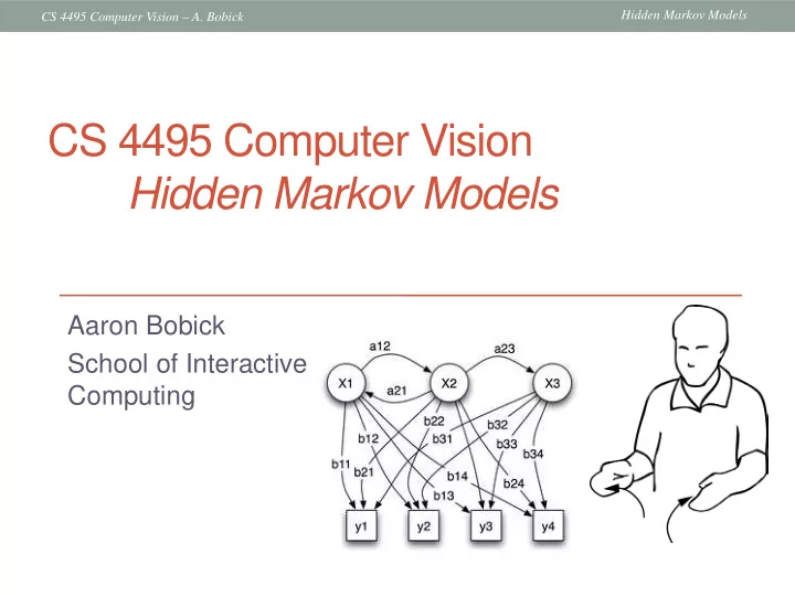
CS 4495 Computer Vision Hidden Markov Models Aaron Bobick School - - PowerPoint PPT Presentation

Hidden Markov Models CS 4495 Computer Vision – A. Bobick

Aaron Bobick School of Interactive Computing

CS 4495 Computer Vision Hidden Markov Models

Hidden Markov Models CS 4495 Computer Vision – A. Bobick

Administrivia

• PS4 – going OK?
• Please share your experiences on Piazza – e.g. discovered

something that is subtle about using vl_sift. If you want to talk about what scales worked and why that’s ok too.

Hidden Markov Models CS 4495 Computer Vision – A. Bobick

Outline

• Time Series
• Markov Models
• Hidden Markov Models
• 3 computational problems of HMMs
• Applying HMMs in vision- Gesture

Slides “borrowed” from UMd and elsewhere Material from: slides from Sebastian Thrun, and Yair Weiss

Hidden Markov Models CS 4495 Computer Vision – A. Bobick

Audio Spectrum

Audio Spectrum of the Song of the Prothonotary Warbler

Hidden Markov Models CS 4495 Computer Vision – A. Bobick

Bird Sounds

Chestnut-sided Warbler Prothonotary Warbler

Hidden Markov Models CS 4495 Computer Vision – A. Bobick

Questions One Could Ask

• What bird is this?
• How will the song

continue?

• Is this bird sick?
• What phases does this

song have?

• Time series classification
• Time series prediction
• Outlier detection
• Time series segmentation

Hidden Markov Models CS 4495 Computer Vision – A. Bobick

Other Sound Samples

Hidden Markov Models CS 4495 Computer Vision – A. Bobick

Another Time Series Problem

Intel Cisco General Electric Microsoft

Hidden Markov Models CS 4495 Computer Vision – A. Bobick

Questions One Could Ask

• Will the stock go up or

down?

• What type stock is this (eg,

risky)?

• Is the behavior abnormal?
• Time series prediction
• Time series classification
• Outlier detection

Hidden Markov Models CS 4495 Computer Vision – A. Bobick

Music Analysis

Hidden Markov Models CS 4495 Computer Vision – A. Bobick

Questions One Could Ask

• Is this Beethoven or Bach?
• Can we compose more of

that?

• Can we segment the piece

into themes?

• Time series classification
• Time series

prediction/generation

• Time series segmentation

Hidden Markov Models CS 4495 Computer Vision – A. Bobick

For vision: Waving, pointing, controlling?

Hidden Markov Models CS 4495 Computer Vision – A. Bobick

The Real Question

• How do we model these problems?
• How do we formulate these questions as a

inference/learning problems?

Hidden Markov Models CS 4495 Computer Vision – A. Bobick

Outline For Today

• Time Series
• Markov Models
• Hidden Markov Models
• 3 computational problems of HMMs
• Applying HMMs in vision- Gesture
• Summary

Hidden Markov Models CS 4495 Computer Vision – A. Bobick

Weather: A Markov Model (maybe?)

Sunny Rainy Snowy 80% 15% 5% 60% 2% 38% 20% 75% 5%

Probability of moving to a given state depends only on the current state: 1st Order Markovian

Hidden Markov Models CS 4495 Computer Vision – A. Bobick

Ingredients of a Markov Model

• States:
• State transition probabilities:
• Initial state distribution:

Sunny Rainy Snowy

80% 15% 5% 60% 2% 38% 20% 75% 5%

1

[ ]

i i

P q S π = =

1 2

{ , ,..., }

N

S S S

1

( | )

ij t i t j

a P q S q S

+

= = =

Hidden Markov Models CS 4495 Computer Vision – A. Bobick

Ingredients of Our Markov Model

• States:
• State transition probabilities:
• Initial state distribution:

(.7 .25 .05) π = { , , }

sunny rainy snowy

S S S

.8 .15 .05 .38 .6 .02 .75 .05 .2 A     =      

Sunny Rainy Snowy

80% 15% 5% 60% 2% 38% 20% 75% 5%

Hidden Markov Models CS 4495 Computer Vision – A. Bobick

Probability of a Time Series

• Given:
• What is the probability of this series?

) 05 . 25 . 7 . ( = π

          = 2 . 05 . 75 . 02 . 6 . 38 . 05 . 15 . 8 . A

0001512 . 2 . 02 . 6 . 6 . 15 . 7 . = ⋅ ⋅ ⋅ ⋅ ⋅ = ) | ( ) | ( ) | ( ) | ( ) | ( ) (

snowy snowy rainy snowy rainy rainy rainy rainy sunny rainy sunny

S S P S S P S S P S S P S S P S P ⋅ ⋅ ⋅ ⋅ ⋅

Hidden Markov Models CS 4495 Computer Vision – A. Bobick

Outline For Today

• Time Series
• Markov Models
• Hidden Markov Models
• 3 computational problems of HMMs
• Applying HMMs in vision- Gesture
• Summary

Hidden Markov Models CS 4495 Computer Vision – A. Bobick

Hidden Markov Models

Sunny Rainy Snowy 80% 15% 5% 60% 2% 38% 20% 75% 5%

Sunny Rainy Snowy

80% 15% 5% 60% 2% 38% 20% 75% 5%

60% 10% 30% 65% 5% 30% 50% 0% 50%

NOT OBSERVABLE OBSERVABLE

Hidden Markov Models CS 4495 Computer Vision – A. Bobick

Probability of a Time Series

• Given:
• What is the probability of this series?

) 05 . 25 . 7 . ( = π

          = 2 . 05 . 75 . 02 . 6 . 38 . 05 . 15 . 8 . A

          = 5 . 5 . 65 . 3 . 05 . 1 . 3 . 6 . B

) ,..., ( ) ,..., | ( ) ( ) | (

7 1 7 1 ,..., all

7 1

q q P q q O P Q P Q O P

q q Q

∑ ∑

= = ) ,..., , , ( ) (

umbrella umbrella coat coat

O O O O P O P =

2 4 6

(0.3 0.1 0.6) (0.7 0.8 ) ... = ⋅ ⋅ ⋅ ⋅ +

Hidden Markov Models CS 4495 Computer Vision – A. Bobick

Specification of an HMM

• N - number of states
• Q = {q1; q2; : : : ;qT} – sequence of states
• Some form of output symbols
• Discrete – finite vocabulary of symbols of size M. One symbol is

“emitted” each time a state is visited (or transition taken).

• Continuous – an output density in some feature space associated

with each state where a output is emitted with each visit

• For a given sequence observation O
• O = {o1; o2; : : : ;oT} – oi observed symbol or feature at time i

Hidden Markov Models CS 4495 Computer Vision – A. Bobick

Specification of an HMM

• A - the state transition probability matrix
• aij = P(qt+1 = j|qt = i)
• B- observation probability distribution
• Discrete: bj(k) = P(ot = k |qt = j) i ≤ k ≤ M
• Continuous bj(x) = p(ot = x | qt = j)
• π - the initial state distribution
• π (j) = P(q1 = j)
• Full HMM over a of states and output space is

thus specified as a triplet: λ = (A,B,π)

S3 S2 S1

Hidden Markov Models CS 4495 Computer Vision – A. Bobick

What does this have to do with Vision?

• Given some sequence of observations, what “model”

generated those?

• Using the previous example: given some observation

sequence of clothing:

• Is this Philadelphia, Boston or Newark?
• Notice that if Boston vs Arizona would not need the

sequence!

Hidden Markov Models CS 4495 Computer Vision – A. Bobick

Outline For Today

• Time Series
• Markov Models
• Hidden Markov Models
• 3 computational problems of HMMs
• Applying HMMs in vision- Gesture
• Summary

Hidden Markov Models CS 4495 Computer Vision – A. Bobick

The 3 great problems in HMM modelling

• 1. Evaluation: Given the model 𝜇 = (𝐵, 𝐶, 𝜌) what is the

probability of occurrence of a particular observation sequence 𝑃 = {𝑝1, … , 𝑝𝑈} = 𝑄(𝑃|𝜇)

• This is the heart of the classification/recognition problem: I have a

trained model for each of a set of classes, which one would most likely generate what I saw.

• 2. Decoding: Optimal state sequence to produce an
• bservation sequence 𝑃 = {𝑝1, … , 𝑝𝑈}
• Useful in recognition problems – helps give meaning to states –

which is not exactly legal but often done anyway.

• 3. Learning: Determine model λ, given a training set of
• bservations
• Find λ, such that 𝑄(𝑃|𝜇) is maximal

Hidden Markov Models CS 4495 Computer Vision – A. Bobick

Problem 1: Naïve solution

NB: Observations are mutually independent, given the hidden

• states. That is, if I know the states then the previous
• bservations don’t help me predict new observation. The

states encode *all* the information. Usually only kind-of true – see CRFs.

) ( )... ( ) ( ) , | ( , | (

2 2 1 1 1 T qT q q t T i t

• b
• b
• b

q

• P

q O P = = ) ∏

=

λ λ

• State sequence 𝑅 = (𝑟1, … 𝑟𝑈)
• Assume independent observations:

Hidden Markov Models CS 4495 Computer Vision – A. Bobick

Problem 1: Naïve solution

1 1 2 2 3 ( 1)

( | ) ...

q q q q q q T qT

P q a a a λ π

−

=

• But we know the probability of any given sequence of

states:

Hidden Markov Models CS 4495 Computer Vision – A. Bobick

Problem 1: Naïve solution

• Given:
• We get:

NB:

• The above sum is over all state paths
• There are 𝑂𝑈 states paths, each ‘costing’

𝑃(𝑈) calculations, leading to 𝑃(𝑈𝑂𝑈) time complexity.

) ( )... ( ) ( ) , | ( , | (

2 2 1 1 1 T qT q q t T i t

• b
• b
• b

q

• P

q O P = = ) ∏

=

λ λ

∑

=

q

q P q O P O P ) | ( ) , | ( ) | ( λ λ λ

1 1 2 2 3 ( 1)

( | ) ...

q q q q q q T qT

P q a a a λ π

−

=

Hidden Markov Models CS 4495 Computer Vision – A. Bobick

• Define auxiliary forward variable α:

Problem 1: Efficient solution

) | , ,..., ( ) (

1

λ α i q

• P

i

t t t

= =

𝛽𝑢(𝑗) is the probability of observing a partial sequence of

• bservables 𝑝1, … 𝑝𝑢 AND at time t, state 𝑟𝑢 = 𝑗

Hidden Markov Models CS 4495 Computer Vision – A. Bobick

Problem 1: Efficient solution

• Recursive algorithm:
• Initialise:
• Calculate:
• Obtain:

1 1

( ) ( )

i i

i b o α π =

1 1 1

( ) ( ) ( )

N t t ij j t i

j i a b o α α

+ + =

  =    

∑

∑

=

=

N i T i

O P

1

) ( ) | ( α λ

Complexity is only O(𝑶𝟑𝑼)!!!

(Partial obs seq to t AND state 𝑗 at 𝑢) x (transition to j at t+1) x (sensor) Sum of different ways

• f getting obs seq

Sum, as can reach 𝑘 from any preceding state

Hidden Markov Models CS 4495 Computer Vision – A. Bobick

The Forward Algorithm (1)

S2 S3 S1 S2 S3 S1 O2 O1 S2 S3 S1 O3 S2 S3 S1 O4 S2 S3 S1 OT

…

) , ,..., ( ) (

1 i t t t

S q O O P i = = α

) ( ) ( ) ( ) | , ( ) , ,..., ( ) , ,..., | , ,..., ( ) , ,..., ( ) (

1 1 1 1 1 1 1 1 1 1 1 1 1 1 1

i a O b i S q S q O P S q O O P S q O O S q O O P S q O O P j

t ij t N i j t i t j t t N i N i i t t i t t j t t j t t t

α α α

+ = + + = = + + + + +

∑ ∑ ∑

= = = = = = = = = =

) ( ) (

1 1

O b i

i i

π α =

(Trellis diagram)

Hidden Markov Models CS 4495 Computer Vision – A. Bobick

Problem 1: Alternative solution

• Define auxiliary

forward variable β:

1 2

( ) ( , ,..., | , )

t t t T t

i P o

• q

i β λ

+ +

= =

Backward algorithm:

β𝑢(𝑗) – the probability of observing a sequence of

• bservables o t+1 , … , 𝑝𝑈 GIVEN state 𝑟𝑢 = 𝑗 at time 𝑢, and λ

Hidden Markov Models CS 4495 Computer Vision – A. Bobick

Problem 1: Alternative solution

• Recursive algorithm:
• Initialize:
• Calculate:
• Terminate:

( ) 1

T j

β =

Complexity is 𝑃(𝑂2𝑈)

1 1 1

( ) ( ) ( )

N t t i j j t j

i j a b o β β +

+ =

= ∑

∑

=

=

N i

i O p

1 1 )

( ) | ( β λ

1 ,..., 1 − = T t

Hidden Markov Models CS 4495 Computer Vision – A. Bobick

Forward-Backward

• Optimality criterion : to choose the states that are

individually most likely at each time t

• The probability of being in state i at time t
• : accounts for partial observation sequence
• account for remainder

t

q

1

( ) ( | , ) ( ) ( ) ( ) ( )

i t t t N t t i

t p q i O i i i i γ λ α β α β

=

= = =

∑

( )

t i

α

( ) :

t i

β

1 2

, ,...

t t T

• +

+

1 2

, ,... t

• o
• = p(O|λ) and qt =i

= p(O|λ)

Hidden Markov Models CS 4495 Computer Vision – A. Bobick

Problem 2: Decoding

• Choose state sequence to maximise probability of
• bservation sequence
• Viterbi algorithm - inductive algorithm that keeps the best

state sequence at each instance

S2 S3 S1 S2 S3 S1 O2 O1 S2 S3 S1 O3 S2 S3 S1 O4 S2 S3 S1 OT

…

Hidden Markov Models CS 4495 Computer Vision – A. Bobick

Problem 2: Decoding

• State sequence to maximize 𝑄(𝑃, 𝑅|฀):
• Define auxiliary variable δ:

1 2

( , ,... | , )

T

P q q q O λ

Viterbi algorithm:

1 2 1 2

( ) max ( , ,..., , , ,... | )

t t t q

i P q q q i o o

• δ

λ = =

𝜀𝑢(𝑗) – the probability of the most probable path ending in state 𝑟𝑢 = 𝑗

Hidden Markov Models CS 4495 Computer Vision – A. Bobick

Problem 2: Decoding

• Recurrent property:
• Algorithm:
• 1. Initialise:

1 1

( ) max( ( ) ) ( )

t t ij j t i

j i a b o δ δ

+ +

=

1 1

( ) ( )

i i

i b o δ π =

N i ≤ ≤ 1

1( )

i ψ =

To get state seq, need to keep track

• f argument to maximise this, for each

t and j. Done via the array 𝜔𝑢(𝑘).

Hidden Markov Models CS 4495 Computer Vision – A. Bobick

Problem 2: Decoding

• 2. Recursion:
• 3. Terminate:

1 1

( ) max( ( ) ) ( )

t t ij j t i N

j i a b o δ δ −

≤ ≤

=

1 1

( ) arg max( ( ) )

t t ij i N

j i a ψ δ −

≤ ≤

=

N j T t ≤ ≤ ≤ ≤ 1 , 2

) ( max

1

i P

T N i

δ

≤ ≤

=

∗

) ( max arg

1

i q

T N i T

δ

≤ ≤ ∗ = P* gives the state-optimized probability Q* is the optimal state sequence (𝑅∗ = {𝑟1∗, 𝑟2∗, … , 𝑟𝑈∗})

Hidden Markov Models CS 4495 Computer Vision – A. Bobick

Problem 2: Decoding

• 4. Backtrack state sequence:

1 1

( )

t t t

q q ψ

∗ ∗ + +

=

1, 2,...,1 t T T = − −

O(N2T) time complexity

S2 S3 S1 S2 S3 S1 O2 O1 S2 S3 S1 O3 S2 S3 S1 O4 S2 S3 S1 OT

…

Hidden Markov Models CS 4495 Computer Vision – A. Bobick

Problem 3: Learning

• Training HMM to encode observation sequence such that

HMM should identify a similar obs seq in future

• Find 𝜇 = (𝐵, 𝐶, 𝜌), maximizing 𝑄(𝑃|𝜇)
• General algorithm:
• Initialize: 𝜇0
• Compute new model 𝜇, using 𝜇0 and observed

sequence 𝑃

• Then
• Repeat steps 2 and 3 until:

λ λ ←

• d

O P O P < − ) | ( log ) | ( log λ λ

Hidden Markov Models CS 4495 Computer Vision – A. Bobick

Problem 3: Learning

) | ( ) ( ) ( ) ( ) , (

1 1

λ β α ξ O P j

• b

a i j i

t t j ij t t + +

=

• Let ξ(i,j) be a probability of being in state i at time t and at

state j at time t+1, given λ and O seq

∑∑

= = + + + +

=

N i N j t t j ij t t t j ij t

j

• b

a i j

• b

a i

1 1 1 1 1 1

) ( ) ( ) ( ) ( ) ( ) ( β α β α

Step 1 of Baum-Welch algorithm:

= p(O and (take i to j) |λ ) = p(O|λ) = p(take i to j at time t |O,λ)

Hidden Markov Models CS 4495 Computer Vision – A. Bobick

Problem 3: Learning

Operations required for the computation

• f the joint event that the system is in state

Si and time t and State Sj at time t+1

Hidden Markov Models CS 4495 Computer Vision – A. Bobick

Problem 3: Learning

Let be a probability of being in state 𝑗 at time 𝑢, given 𝑃

• expected no. of transitions from state i
• expected no. of transitions

1

( ) ( , )

N t t j

i i j γ ξ

=

= ∑

1 1

( )

T t t

i γ

− =

∑

1 1

( , )

T t t

i j ξ

− =

∑

j i →

( )

t i

γ

Hidden Markov Models CS 4495 Computer Vision – A. Bobick

Problem 3: Learning

the expected frequency of state i at time t=1 ratio of expected no. of transitions from state i to j over expected no. of transitions from state i ratio of expected no. of times in state j observing symbol k over expected no. of times in state j

∑ ∑

= ) ( ) , ( ˆ i j i a

t t ij

γ ξ

Step 2 of Baum-Welch algorithm:

,

( ) ˆ ( ) ( )

t

t t o k j t

j b k j γ γ

=

= ∑

∑

) ( ˆ

1 i

γ π =

Hidden Markov Models CS 4495 Computer Vision – A. Bobick

Problem 3: Learning

• Baum-Welch algorithm uses the forward and backward

algorithms to calculate the auxiliary variables 𝛽, 𝛾

• B-W algorithm is a special case of the EM algorithm:
• E-step: calculation of ξ and γ
• M-step: iterative calculation of , ,
• Practical issues:
• Can get stuck in local maxima
• Numerical problems – log and scaling

π ˆ

ij

a ˆ

) ( ˆ k bj

Hidden Markov Models CS 4495 Computer Vision – A. Bobick

Now HMMs and Vision: Gesture Recognition…

Hidden Markov Models CS 4495 Computer Vision – A. Bobick

"Gesture recognition"-like activities

Hidden Markov Models CS 4495 Computer Vision – A. Bobick

Some thoughts about gesture

• There is a conference on Face and Gesture Recognition

so obviously Gesture recognition is an important problem…

• Prototype scenario:
• Subject does several examples of "each gesture"
• System "learns" (or is trained) to have some sort of model for each
• At run time compare input to known models and pick one
• New found life for gesture recognition:

Hidden Markov Models CS 4495 Computer Vision – A. Bobick

Generic Gesture Recognition using HMMs

Nam, Y., & Wohn, K. (1996, July). Recognition of space-time hand-gestures using hidden Markov model. In ACM symposium on Virtual reality software and technology (pp. 51-58).

Hidden Markov Models CS 4495 Computer Vision – A. Bobick

Generic gesture recognition using HMMs (1)

Data glove

Hidden Markov Models CS 4495 Computer Vision – A. Bobick

Generic gesture recognition using HMMs (2)

Hidden Markov Models CS 4495 Computer Vision – A. Bobick

Generic gesture recognition using HMMs (3)

Hidden Markov Models CS 4495 Computer Vision – A. Bobick

Generic gesture recognition using HMMs (4)

Hidden Markov Models CS 4495 Computer Vision – A. Bobick

Generic gesture recognition using HMMs (5)

Hidden Markov Models CS 4495 Computer Vision – A. Bobick

Wins and Losses of HMMs in Gesture

• Good points about HMMs:
• A learning paradigm that acquires spatial and temporal models and

does some amount of feature selection.

• Recognition is fast; training is not so fast but not too bad.
• Not so good points:
• If you know something about state definitions, difficult to

incorporate

• Every gesture is a new class, independent of anything else you’ve

learned.

• ->Particularly bad for “parameterized gesture.”

Hidden Markov Models CS 4495 Computer Vision – A. Bobick

Parameterized Gesture

“I caught a fish this big.”

Hidden Markov Models CS 4495 Computer Vision – A. Bobick

Parametric HMMs (PAMI, 1999)

• Basic ideas:
• Make output probabilities of the state be a function of the parameter of

interest, 𝑐𝑘 (𝒚) becomes 𝑐′

𝑘(𝒚, 𝜄).

• Maintain same temporal properties, 𝑏𝑗𝑘 unchanged.
• Train with known parameter values to solve for dependencies of 𝑐𝑐 on θ.
• During testing, use EM to find θ that gives the highest probability. That

probability is confidence in recognition; best θ is the parameter.

• Issues:
• How to represent dependence
• n θ ?
• How to train given θ ?
• How to test for θ ?
• What are the limitations on

dependence on θ ?

Hidden Markov Models CS 4495 Computer Vision – A. Bobick

Linear PHMM - Representation

Represent dependence on θ as linear movement of the mean of the Gaussians of the states: Need to learn Wj and µj for each state j. (ICCV ’98)

Hidden Markov Models CS 4495 Computer Vision – A. Bobick

Linear PHMM - training

• Need to derive EM equations for linear parameters and

proceed as normal:

Hidden Markov Models CS 4495 Computer Vision – A. Bobick

Linear HMM - testing

• Derive EM equations with respect to θ :
• We are testing by EM! (i.e. iterative):
• Solve for γtk given guess for θ
• Solve for θ given guess for γtk

Hidden Markov Models CS 4495 Computer Vision – A. Bobick

How big was the fish?

Hidden Markov Models CS 4495 Computer Vision – A. Bobick

Pointing

• Pointing is the prototypical

example of a parameterized gesture.

• Assuming two DOF, can

parameterize either by (x,y) or by (θ,φ) .

• Under linear assumption must

choose carefully.

• A generalized non-linear map

would allow greater freedom. (ICCV 99)

Hidden Markov Models CS 4495 Computer Vision – A. Bobick

Linear pointing results

Test for both recognition and recovery: If prune based on legal θ (MAP via uniform density) :

Hidden Markov Models CS 4495 Computer Vision – A. Bobick

Noise sensitivity

• Compare ad hoc procedure with PHMM parameter

recovery (ignoring “their” recognition problem!!).

Hidden Markov Models CS 4495 Computer Vision – A. Bobick

HMMs and vision

• HMMs capture sequencing nicely in a probabilistic

manner.

• Moderate time to train, fast to test.
• More when we do activity recognition…