CS 4495 Computer Vision Motion Models Aaron Bobick School of - - PowerPoint PPT Presentation

Motion models CS 4495 Computer Vision – A. Bobick

Aaron Bobick School of Interactive Computing

CS 4495 Computer Vision Motion Models

Motion models CS 4495 Computer Vision – A. Bobick

Outline

• Last time: dense motion: optic flow
• Brightness constancy constraint equation
• Lucas-Kanade
• 2D Motion models
• Bergen, ’92
• Pyramids
• Layers
• Motion fields from 3D motions
• Parametric motion

Motion models CS 4495 Computer Vision – A. Bobick

Visual motion

Many slides adapted from S. Seitz, R. Szeliski, M. Pollefeys, K. Grauman and others…

Motion models CS 4495 Computer Vision – A. Bobick

Motion estimation: Optical flow

Will start by estimating motion of each pixel separately Then will consider motion of entire image

Motion models CS 4495 Computer Vision – A. Bobick

Problem definition: optical flow

How to estimate pixel motion from image I(x,y,t) to I(x,y,t) ?

• Solve pixel correspondence problem

– given a pixel in I(x,y,t), look for nearby pixels of the same color in I(x,y,t+1)

Key assumptions

• color constancy: a point in I(x,y, looks the same in I(x,y,t+1)

– For grayscale images, this is brightness constancy

• small motion: points do not move very far

This is called the optical flow problem

( , , ) I x y t ( , , 1) I x y t +

Motion models CS 4495 Computer Vision – A. Bobick

( , , 1) ( , , ) ( , , 1) ( , , ) [ ( , , 1) ( , )] ,

x y x y t x y t

I x u y v t I x y t I x y t I u I v I x y t I x y t I x y I u I v I I u I v I I u v = + + + − ≈ + + + − ≈ + − + + ≈ + + ≈ + ∇ ⋅ < >

Optical flow equation

• Combining these two equations

In the limit as u and v go to zero, this becomes exact Brightness constancy constraint equation

x y t

I u I v I + + =

,

t

I I u v = + ∇ ⋅ < >

Motion models CS 4495 Computer Vision – A. Bobick

Optical flow equation

• Q: how many unknowns and equations per pixel?

Intuitively, what does this constraint mean?

• The component of the flow in the gradient direction is determined
• The component of the flow parallel to an edge is unknown

2 unknowns, one equation edge (u,v) (u’,v’) gradient (u+u’,v+v’)

x y t

I u I v I + + =

,

t

I I u v = + ∇ ⋅ < >

• r

Motion models CS 4495 Computer Vision – A. Bobick

Aperture problem

Motion models CS 4495 Computer Vision – A. Bobick

Solving the aperture problem

• How to get more equations for a pixel?
• Basic idea: impose additional constraints
• most common is to assume that the flow field is smooth locally
• one method: pretend the pixel’s neighbors have the same (u,v)
• If we use a 5x5 window, that gives us 25 equations per pixel!

Motion models CS 4495 Computer Vision – A. Bobick

Lukas-Kanade flow

• Prob: we have more equations than unknowns
• The summations are over all pixels in the K x K window
• This technique was first proposed by Lukas & Kanade (1981)
• minimum least squares solution given by solution (in d) of:

Solution: solve least squares problem

Motion models CS 4495 Computer Vision – A. Bobick

Eigenvectors of A

TA

• Recall the Harris corner detector: M = ATA is the

second moment matrix

• The eigenvectors and eigenvalues of M relate to

edge direction and magnitude

• The eigenvector associated with the larger eigenvalue points in the

direction of fastest intensity change

• The other eigenvector is orthogonal to it

Motion models CS 4495 Computer Vision – A. Bobick

Violating assumptions in Lucas-Kanade

• The motion is large (larger than a pixel)
• Not-linear: Iterative refinement
• Local minima: coarse-to-fine estimation
• A point does not move like its neighbors
• Motion segmentation
• Brightness constancy does not hold
• Do exhaustive neighborhood search with normalized correlation -

tracking features – maybe SIFT – more later….

Motion models CS 4495 Computer Vision – A. Bobick

Violating assumptions in Lucas-Kanade

• The motion is large (larger than a pixel)
• Not-linear: Iterative refinement
• Local minima: coarse-to-fine estimation
• A point does not move like its neighbors
• Motion segmentation
• Brightness constancy does not hold
• Do exhaustive neighborhood search with normalized correlation -

tracking features – maybe SIFT – more later….

Motion models CS 4495 Computer Vision – A. Bobick

Not tangent: Iterative Refinement

Iterative Lukas-Kanade Algorithm

1.

Estimate velocity at each pixel by solving Lucas-Kanade equations

2.

Warp It towards It+1 using the estimated flow field

• use image warping techniques

3.

Repeat until convergence

Motion models CS 4495 Computer Vision – A. Bobick

Optical Flow: Iterative Estimation

x x0

Initial guess: Estimate: estimate update

(using d for displacement here instead of u)

Motion models CS 4495 Computer Vision – A. Bobick

Optical Flow: Iterative Estimation

x x0

estimate update Initial guess: Estimate:

Motion models CS 4495 Computer Vision – A. Bobick

Optical Flow: Iterative Estimation

x x0

Initial guess: Estimate: Initial guess: Estimate: estimate update

Motion models CS 4495 Computer Vision – A. Bobick

Optical Flow: Iterative Estimation

x x0

Motion models CS 4495 Computer Vision – A. Bobick

Revisiting the small motion assumption

• Is this motion small enough?
• Probably not—it’s much larger than one pixel (2nd order terms dominate)
• How might we solve this problem?

Motion models CS 4495 Computer Vision – A. Bobick

Optical Flow: Aliasing

Temporal aliasing causes ambiguities in optical flow because images can have many pixels with the same intensity. I.e., how do we know which ‘correspondence’ is correct?

nearest match is correct (no aliasing) nearest match is incorrect (aliasing)

To overcome aliasing: coarse-to-fine estimation.

actual shift estimated shift

Motion models CS 4495 Computer Vision – A. Bobick

Reduce the resolution!

Motion models CS 4495 Computer Vision – A. Bobick

image 2 image 1

Gaussian pyramid of image 1 Gaussian pyramid of image 2 image 2 image 1

u=10 pixels u=5 pixels u=2.5 pixels u=1.25 pixels

Coarse-to-fine optical flow estimation

Motion models CS 4495 Computer Vision – A. Bobick

image I image J

Gaussian pyramid of image 1 Gaussian pyramid of image 2 image 2 image 1

Coarse-to-fine optical flow estimation

run iterative L-K

run iterative L-K warp

warp & upsample Upsample flow

. . .

Motion models CS 4495 Computer Vision – A. Bobick

Multi-scale

Motion models CS 4495 Computer Vision – A. Bobick

Remember: Image sub-sampling

Throw away every other row and column to create a 1/2 size image

• called image sub-sampling

1/4 1/8

• S. Seitz

Motion models CS 4495 Computer Vision – A. Bobick

Bad image sub-sampling

1/4 (2x zoom) 1/8 (4x zoom) Aliasing! What do we do? 1/2

• S. Seitz

Motion models CS 4495 Computer Vision – A. Bobick

Gaussian (lowpass) pre-filtering

G 1/4 G 1/8 Gaussian 1/2

Solution: filter the image, then subsample

• S. Seitz

Motion models CS 4495 Computer Vision – A. Bobick

Subsampling with Gaussian pre-filtering

G 1/4 G 1/8 Gaussian 1/2

• S. Seitz

Motion models CS 4495 Computer Vision – A. Bobick

Band-pass filtering

Gaussian Pyramid (low-pass images)

These are “bandpass” images (almost).

Laplacian Pyramid (subband images)

Motion models CS 4495 Computer Vision – A. Bobick

Laplacian Pyramid

• How can we reconstruct (collapse) this

pyramid into the original image?

Need this! Original image

Motion models CS 4495 Computer Vision – A. Bobick

Image Pyramids

Known as a Gaussian Pyramid [Burt and Adelson, 1983]

• S. Seitz

Motion models CS 4495 Computer Vision – A. Bobick

Computing the Laplacian Pyramid

Need Gk to reconstruct Reduce Expand

Motion models CS 4495 Computer Vision – A. Bobick

Reduce and Expand

Reduce Apply “5-tap” separable filter to make reduced image.

Motion models CS 4495 Computer Vision – A. Bobick

Reduce and Expand

Reduce Expand Apply “5-tap” separable filter to make reduced image. Apply different “3-tap” separable filters for even and odd pixels to make expanded image...

Motion models CS 4495 Computer Vision – A. Bobick

Just Expand

Apply different “3-tap” separable filters for even and

• dd pixels to make expanded image.

Even Odd Coarser Finer

Motion models CS 4495 Computer Vision – A. Bobick

What can you do with band limited imaged?

Motion models CS 4495 Computer Vision – A. Bobick

Apples and Oranges in bandpass

L0 L2 L4 Reconstructed

Motion models CS 4495 Computer Vision – A. Bobick

Applying pyramids to LK

Motion models CS 4495 Computer Vision – A. Bobick

Coarse-to-fine global motion estimation

Reduce Reduce Reduce Reduce

LK LK LK Warp Warp Warp x2 Expand x2 Expand

Final <u(x,y), v(x,y)>

x2 Expand

Motion models CS 4495 Computer Vision – A. Bobick

Multi-resolution Lucas Kanade Algorithm

Compute Iterative LK at highest level Initialize 𝑣𝐿+1, 𝑤𝐿+1 = 0 at size of level K+1 For Each Level i from K to 0

• Upsample 𝑣𝑗+1, 𝑤𝑗+1 to create 𝑣𝑗

𝑞, 𝑤𝑗 𝑞flow fields of now twice

resolution as level i+1.

• Multiply 𝑣𝑗

𝑞, 𝑤𝑗 𝑞 by 2 to get predicted flow

• Warp 𝐽2 according to predicted flow
• Compute It –temporal derivative
• Apply LK to get 𝑣𝑗

𝜀, 𝑤𝑗 𝜀 (the correction in flow)

• Add corrections to obtain the flow u(i), v(i) at ith level, i.e.,

𝑣𝑗 = 𝑣𝑗

𝑞 + 𝑣𝑗 𝜀; 𝑤𝑗 = 𝑤𝑗 𝑞 + 𝑤𝑗 𝜀

Motion models CS 4495 Computer Vision – A. Bobick

Optical Flow Results

* From Khurram Hassan-Shafique CAP5415 Computer Vision 2003

Motion models CS 4495 Computer Vision – A. Bobick

Optical Flow Results

* From Khurram Hassan-Shafique CAP5415 Computer Vision 2003

Motion models CS 4495 Computer Vision – A. Bobick

Moving to models

• Previous method(s) give dense flow with little or no

constraint between locations (smoothness is either explicit

• r implicit).
• Suppose you “know” that motion is constrained, e.g.
• Small rotation about horizontal or vertical axis (or both) that is very

close to a translation.

• Distant independent moving objects
• In this case you might “model” the flow…

Ready for another old slide?

Motion models CS 4495 Computer Vision – A. Bobick

Motion models

Translation 2 unknowns Similarity 4 unknowns Perspective 8 unknowns Affine 6 unknowns

Motion models CS 4495 Computer Vision – A. Bobick

Focus of Expansion (FOE) - Example

Motion models CS 4495 Computer Vision – A. Bobick

Full motion model

• From physics or elsewhere:

[ ]

          − − − =

1 2 1 3 2 3

a a a a a a ax

V R T = Ω× +

          +                     − − − ≈          

Z Y x

T T T X Y X Z Y Z Z Y X

V V V Z Y X V V V ω ω ω ω ω ω

=          

Z Y X

V V V =          

Z Y X

T T T

V V V =          

Z Y X

ω ω ω

Velocity Vector

Translational Component of Velocity Angular Velocity

Motion models CS 4495 Computer Vision – A. Bobick

General motion

Z V y Z V f Z V Z Y f Z V f Z YV ZV f v v Z V x Z V f Z V Z X f Z V f Z XV ZV f v u

Z Y Z Y Z Y y Z X Z X Z X x

− =       − = − = = − =       − = − = =

2 2

Z Y f y Z X f x = =

( , ) 1 ( , ) ( , ) ( , ) ( , ) u x y x y x y v x y Z x y   = +     A T B Ω

Take derivatives: ( , ) f x x y f y −   =   −   A

2 2

( ) / ( ) / ( , ) ( ) / ( ) / xy f f x f y x y f y f xy f x   − + =   + − −   B

Where T is translation vector, Ω is rotation Why is Z only here?

Motion models CS 4495 Computer Vision – A. Bobick

If a plane and perspective… aX bY cZ d + + + =

2 1 2 3 7 8 2 4 5 6 7 8

( , ) ( , ) u x y a a x a y a x a xy v x y a a x a y a xy a y = + + + + = + + + +

Motion models CS 4495 Computer Vision – A. Bobick

If a plane and orthographic…

1 2 3 4 5 6

( , ) ( , ) u x y a a x a y v x y a a x a y = + + = + +

Affine!

Motion models CS 4495 Computer Vision – A. Bobick

) ( ) (

6 5 4 3 2 1

≈ + + + + + +

t y x

I y a x a a I y a x a a I

• Substituting into the brightness constancy

equation: y a x a a y x v y a x a a y x u

6 5 4 3 2 1

) , ( ) , ( + + = + + =

• Each pixel provides 1 linear constraint in

6 unknowns

[ ]

2

∑

+ + + + + + =

t y x

I y a x a a I y a x a a I a Err ) ( ) ( ) (

6 5 4 3 2 1



• Least squares minimization:

Affine motion

≈ + ⋅ + ⋅

t y x

I v I u I

Motion models CS 4495 Computer Vision – A. Bobick

Affine motion

• Can sum gradients over window or entire image:
• Minimize squared error (robustly)
• This is an example of parametric flow – can substitute

any linear model easily. Others with some work.

[ ]

2

∑

+ + + + + + =

t y x

I y a x a a I y a x a a I a Err ) ( ) ( ) (

6 5 4 3 2 1



1 1 1 1 1 1 2 2 2 2 2 2 3 4 5 6 x x x y y y t x x x y y y t n x x n x n y y n y n t

a I I x I y I I x I y I a I I x I y I I x I y I a a a I I x I y I I x I y I a                         ⋅ = −                                

Motion models CS 4495 Computer Vision – A. Bobick

Hierarchical model-based flow

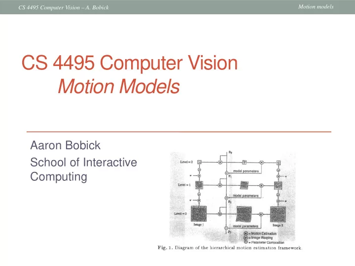
James R. Bergen, P. Anandan, Keith J. Hanna, Rajesh Hingorani: “Hierarchical Model-Based Motion Estimation," ECCV 1992: 237-252

Motion models CS 4495 Computer Vision – A. Bobick

Now, if different motion regions…

Motion models CS 4495 Computer Vision – A. Bobick

Layered motion

• Basic idea: break image sequence into “layers” each of

which has a coherent motion

• J. Wang and E. Adelson. Layered Representation for Motion Analysis. CVPR 1993.

Motion models CS 4495 Computer Vision – A. Bobick

What are layers?

• Each layer is defined by an alpha mask and an affine

motion model

• J. Wang and E. Adelson. Layered Representation for Motion Analysis. CVPR 1993.

Motion models CS 4495 Computer Vision – A. Bobick

y a x a a y x v y a x a a y x u

6 5 4 3 2 1

) , ( ) , ( + + = + + =

Local flow estimates

Motion segmentation with an affine model

• J. Wang and E. Adelson. Layered Representation for Motion Analysis. CVPR 1993.

Motion models CS 4495 Computer Vision – A. Bobick

Motion segmentation with an affine model

y a x a a y x v y a x a a y x u

6 5 4 3 2 1

) , ( ) , ( + + = + + =

Equation of a plane (parameters a1, a2, a3 can be found by least squares)

• J. Wang and E. Adelson. Layered Representation for Motion Analysis. CVPR 1993.

Motion models CS 4495 Computer Vision – A. Bobick

Motion segmentation with an affine model

y a x a a y x v y a x a a y x u

6 5 4 3 2 1

) , ( ) , ( + + = + + =

1D example

u(x,y) Local flow estimate Segmented estimate Line fitting

Equation of a plane (parameters a1, a2, a3 can be found by least squares)

True flow “Foreground” “Background” Occlusion

• J. Wang and E. Adelson. Layered Representation for Motion Analysis. CVPR 1993.

Motion models CS 4495 Computer Vision – A. Bobick

How do we estimate the layers?

• Compute local flow in a coarse-to-fine fashion
• Obtain a set of initial affine motion hypotheses
• Divide the image into blocks and estimate affine motion

parameters in each block by least squares

• Eliminate hypotheses with high residual error
• Perform k-means clustering on affine motion parameters
• Merge clusters that are close and retain the largest clusters to
• btain a smaller set of hypotheses to describe all the motions in

the scene

• Iterate until convergence:
• Assign each pixel to best hypothesis
• Pixels with high residual error remain unassigned
• Perform region filtering to enforce spatial constraints
• Re-estimate affine motions in each region
• J. Wang and E. Adelson. Layered Representation for Motion Analysis. CVPR 1993.

Motion models CS 4495 Computer Vision – A. Bobick

Example result

• J. Wang and E. Adelson. Layered Representation for Motion Analysis. CVPR 1993.

Motion models CS 4495 Computer Vision – A. Bobick

Recovering image motion

• Feature-based methods (e.g. SIFT, Ransac, regression)
• Extract visual features (corners, textured areas) and track them -

sometimes over multiple frames

• Sparse motion fields, but possibly robust tracking
• Good for global motion
• Suitable especially when image motion is large (10-s of pixels)
• PS4!
• Direct-methods (e.g. optical flow)
• Directly recover image motion from spatio-temporal image

brightness variations

• Dense, local motion fields, but more sensitive to appearance

variations

• Suitable for video and when image motion is small (< 10 pixels)
• PS5!!!