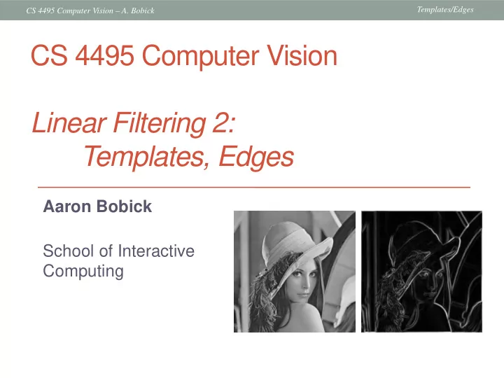
CS 4495 Computer Vision Linear Filtering 2: Templates, Edges Aaron - - PowerPoint PPT Presentation

Templates/Edges CS 4495 Computer Vision – A. Bobick

Aaron Bobick School of Interactive Computing

CS 4495 Computer Vision Linear Filtering 2: Templates, Edges

Templates/Edges CS 4495 Computer Vision – A. Bobick

Last time: Convolution

• Convolution:
• Flip the filter in both dimensions (right to left, bottom to top)
• Then apply cross-correlation

Notation for convolution

• perator

H* F

• K. Grauman

H*

G H F = ∗

Templates/Edges CS 4495 Computer Vision – A. Bobick

Convolution vs. correlation

Convolution (Cross-)correlation

• When H is symmetric, no difference. We tend to use the terms

interchangeably.

• Convolution with an impulse (centered at 0,0) is the identity
• K. Grauman

G H F = ∗

Templates/Edges CS 4495 Computer Vision – A. Bobick

Filters for features

• Previously, thinking of filtering

as a way to remove or reduce noise

• Now, consider how filters will

allow us to abstract higher- level “features”.

• Map raw pixels to an intermediate

representation that will be used for subsequent processing

• Goal: reduce amount of data,

discard redundancy, preserve what’s useful

• K. Grauman

Templates/Edges CS 4495 Computer Vision – A. Bobick

Template matching

• Filters as templates:

Note that filters look like the effects they are intended to find --- “matched filters”

• Use (normalized) cross-correlation score to find a given

pattern (template) in the image.

• Normalization needed to control for relative brightness. More in

problem sets.

• K. Grauman

Templates/Edges CS 4495 Computer Vision – A. Bobick

Template matching

Scene Template (mask)

A toy example

• K. Grauman

Templates/Edges CS 4495 Computer Vision – A. Bobick

Template matching

Template Detected template

• K. Grauman

Templates/Edges CS 4495 Computer Vision – A. Bobick

Template matching

Detected template Correlation map

• K. Grauman

Templates/Edges CS 4495 Computer Vision – A. Bobick

Where’s Waldo?

Scene Template

• K. Grauman

Templates/Edges CS 4495 Computer Vision – A. Bobick

Where’s Waldo?

Detected template Template

• K. Grauman

Templates/Edges CS 4495 Computer Vision – A. Bobick

Template demo…

• In directory C:\Bobick\matlab\CS4495\Filter
• echodemo waldotemplate

Templates/Edges CS 4495 Computer Vision – A. Bobick

Where’s Waldo?

Detected template Correlation map

• K. Grauman

Templates/Edges CS 4495 Computer Vision – A. Bobick

Template matching

Scene Template

What if the template is not identical to some subimage in the scene?

• K. Grauman

Templates/Edges CS 4495 Computer Vision – A. Bobick

Template matching

Detected template Template

Match can be meaningful, if scale, orientation, and general appearance is right.

• K. Grauman

Templates/Edges CS 4495 Computer Vision – A. Bobick

Generic features…

• When looking for a specific object or pattern, the features

can be defined for that pattern – we will do this later in the course for specific object recognition.

• But for generic images, what would be good features?

What are the parts or properties of the image that encode its “meaning” for human (or other biological) observers?

• Some examples of greatly reduced images…

Templates/Edges CS 4495 Computer Vision – A. Bobick

Edges seem to be important…

Templates/Edges CS 4495 Computer Vision – A. Bobick

Origin of Edges

• Edges are caused by a variety of factors
• Information theory view: edges encode change, change

is what is hard to predict, therefore edges efficiently encode an image

depth discontinuity surface color discontinuity illumination discontinuity surface normal discontinuity

Templates/Edges CS 4495 Computer Vision – A. Bobick

In a real image

Depth discontinuity:

• bject boundary

Change in surface

• rientation: shape

Cast shadows Reflectance change: appearance information, texture

Templates/Edges CS 4495 Computer Vision – A. Bobick

Contrast and invariance

Templates/Edges CS 4495 Computer Vision – A. Bobick

Edge detection

• Convert a 2D image into a set of curves
• Extracts salient features of the scene
• More compact than pixels

Templates/Edges CS 4495 Computer Vision – A. Bobick

Edge detection

• How can you tell that a pixel is on an edge?

Templates/Edges CS 4495 Computer Vision – A. Bobick

Images as functions…

• Edges look like steep cliffs

Templates/Edges CS 4495 Computer Vision – A. Bobick

Edge Detection

Basic idea: look for a neighborhood with strong signs of change. 81 82 26 24 82 33 25 25 81 82 26 24 Problems:

• neighborhood size
• how to detect change

Templates/Edges CS 4495 Computer Vision – A. Bobick

Derivatives and edges

image intensity function (along horizontal scanline) first derivative edges correspond to extrema of derivative

Source: L. Lazebnik

An edge is a place of rapid change in the image intensity function.

Templates/Edges CS 4495 Computer Vision – A. Bobick

Differential Operators

• Differential operators – here we mean some operation that when

applied to the image returns some derivatives.

• We will model these “operators” as masks/kernels which when

applied to the image yields a new function that is the image gradient function.

• We will then threshold the this gradient function to select the

edge pixels.

• Which brings us to the question:

What’s a gradient?

Templates/Edges CS 4495 Computer Vision – A. Bobick

Image gradient

The gradient of an image: The gradient direction is given by:

• how does this relate to the direction of the edge?

The edge strength is given by the gradient magnitude The gradient points in the direction of most rapid increase in intensity

Templates/Edges CS 4495 Computer Vision – A. Bobick

Discrete gradient

For 2D function, f(x,y), the partial derivative is: For discrete data, we can approximate using finite differences:

ε ε

ε

) , ( ) , ( lim ) , ( y x f y x f x y x f − + = ∂ ∂

→

1 ) , ( ) , 1 ( ) , ( y x f y x f x y x f − + ≈ ∂ ∂ ( 1, ) ( , ) f x y f x y ≈ + −

“right derivative” But is it???

Templates/Edges CS 4495 Computer Vision – A. Bobick

Computer Vision - A Modern Approach Set: Linear Filters Slides by D.A. Forsyth

Finite differences

Templates/Edges CS 4495 Computer Vision – A. Bobick

Partial derivatives of an image

Which shows changes with respect to x?

• 1

1 1

• 1
• r

?

• 1 1

x y x f ∂ ∂ ) , ( y y x f ∂ ∂ ) , (

(showing correlation filters)

Templates/Edges CS 4495 Computer Vision – A. Bobick

Differentiation and convolution

• For 2D function, f(x,y), the partial derivative is:
• For discrete data, we can approximate using finite

differences:

• To implement above as convolution, what would be the

associated filter?

ε ε

ε

) , ( ) , ( lim ) , ( y x f y x f x y x f − + = ∂ ∂

→

1 ) , ( ) , 1 ( ) , ( y x f y x f x y x f − + ≈ ∂ ∂

Templates/Edges CS 4495 Computer Vision – A. Bobick

The discrete gradient

• We want an “operator” (mask/kernel) that we can apply to

the image that implements: How would you implement this as a cross-correlation?

(not flipped)

• 1/2 0 +1/2
• 1

+1

Not symmetric around image point; which is “middle” pixel? Average of “left” and “right” derivative . See?

ε ε

ε

) , ( ) , ( lim ) , ( y x f y x f x y x f − + = ∂ ∂

→

Templates/Edges CS 4495 Computer Vision – A. Bobick

On a pixel of the image I

• Let gx be the response to mask Sx (sometimes * 1/8)
• Let gy be the response to mask Sy

What is the gradient? g = (gx

2 + gy 2)1/2 is the gradient magnitude.

θ = atan2(gy , gx) is the gradient direction. (Sobel) Gradient is ∇I = [gx gy]T

• 1

1

• 2

2

• 1

1 1 2 1

• 1 -2 -1

Example: Sobel operator

Templates/Edges CS 4495 Computer Vision – A. Bobick

• riginal image gradient thresholded

magnitude gradient magnitude

Sobel Operator on Blocks Image

Templates/Edges CS 4495 Computer Vision – A. Bobick

Some Well-Known Masks for Computing Gradients

• Sobel:
• Prewitt:
• Roberts
• 1 0 1
• 1 0 1
• 1 0 1

1 1 1 0 0 0

• 1 -1 -1
• 1 0 1
• 2 0 2
• 1 0 1

1 2 1 0 0 0

• 1 -2 -1

0 1

• 1 0

1 0 0 -1 Sx Sy

Templates/Edges CS 4495 Computer Vision – A. Bobick

Matlab does edges

>> My = fspecial(‘sobel’); >> outim = imfilter(double(im), My); >> imagesc(outim); >> colormap gray;

Templates/Edges CS 4495 Computer Vision – A. Bobick

But…

• Consider a single row or column of the image
• Plotting intensity as a function of x
• Apply derivative operator….

Uh, where’s the edge?

Templates/Edges CS 4495 Computer Vision – A. Bobick

Finite differences responding to noise

Increasing noise -> (this is zero mean additive gaussian noise)

• D. Forsyth

Templates/Edges CS 4495 Computer Vision – A. Bobick

Where is the edge?

Solution: smooth first

Look for peaks in

f h h f ∗ ) (

x h

f

∂ ∂

∗

) (

x h

f

∂ ∂

∗

Templates/Edges CS 4495 Computer Vision – A. Bobick

Derivative theorem of convolution

• This saves us one operation:

How can we find (local) maxima of a function?

) ( ) (

x x

h f h f

∂ ∂ ∂ ∂

∗ = ∗

f h

x h ∂ ∂

( )

x h

f

∂ ∂

∗

Templates/Edges CS 4495 Computer Vision – A. Bobick

2nd derivative of Gaussian

• Consider

Second derivative of Gaussian

• perator

Where is the edge? Zero-crossings of bottom graph

2 2 (

)

x

h f

∂ ∂

∗

2 2 x h ∂ ∂ 2 2 (

)

x

h f

∂ ∂

∗ f

x h ∂ ∂

Templates/Edges CS 4495 Computer Vision – A. Bobick

What about 2D?

Templates/Edges CS 4495 Computer Vision – A. Bobick

Derivative of Gaussian filter

[ ]

1 1 − ⊗

[ ]

0.0030 0.0133 0.0219 0.0133 0.0030 0.0133 0.0596 0.0983 0.0596 0.0133 0.0219 0.0983 0.1621 0.0983 0.0219 0.0133 0.0596 0.0983 0.0596 0.0133 0.0030 0.0133 0.0219 0.0133 0.0030

) ( ) ( h g I h g I ⊗ ⊗ = ⊗ ⊗

Why is this preferable?

Templates/Edges CS 4495 Computer Vision – A. Bobick

Derivative of Gaussian filters

x-direction y-direction

Source: L. Lazebnik

Is this for correlation

• r convolution?

And for y it’s always a problem!

Templates/Edges CS 4495 Computer Vision – A. Bobick

Smoothing with a Gaussian

for sigma=1:3:10 h = fspecial('gaussian‘, fsize, sigma);

• ut = imfilter(im, h);

imshow(out); pause; end

…

Parameter σ is the “scale” / “width” / “spread” of the Gaussian kernel, and controls the amount of smoothing.

Templates/Edges CS 4495 Computer Vision – A. Bobick

Smoothing with a Gaussian

Recall: parameter σ is the “scale” / “width” / “spread” of the Gaussian kernel, and controls the amount of smoothing.

…

Templates/Edges CS 4495 Computer Vision – A. Bobick

Effect of σ on derivatives

The apparent structures differ depending on Gaussian’s scale parameter. Larger values: larger scale edges detected Smaller values: finer features detected

σ = 1 pixel σ = 3 pixels

Templates/Edges CS 4495 Computer Vision – A. Bobick

Gradients -> edges

• Primary edge detection steps:
• 1. Smoothing: suppress noise
• 2. Edge “enhancement”: filter for contrast
• 3. Edge localization
• Determine which local maxima from filter output are actually edges
• vs. noise
• Threshold, Thin

Templates/Edges CS 4495 Computer Vision – A. Bobick

Canny edge detector

• Filter image with derivative of Gaussian
• Find magnitude and orientation of gradient
• Non-maximum suppression:
• Thin multi-pixel wide “ridges” down to single pixel

width

• Linking and thresholding (hysteresis):
• Define two thresholds: low and high
• Use the high threshold to start edge curves and the

low threshold to continue them

• MATLAB: edge(image, ‘canny’);
• >>help edge

Source: D. Lowe, L. Fei-Fei

Templates/Edges CS 4495 Computer Vision – A. Bobick

The Canny edge detector

• riginal image (Lena)

Templates/Edges CS 4495 Computer Vision – A. Bobick

The Canny edge detector

magnitude of the gradient

Templates/Edges CS 4495 Computer Vision – A. Bobick

The Canny edge detector

thresholding

Templates/Edges CS 4495 Computer Vision – A. Bobick

The Canny edge detector

thinning (non-maximum suppression) Problem: pixels along this edge didn’t survive the thresholding

Templates/Edges CS 4495 Computer Vision – A. Bobick

The Canny edge detector

thresholding How to turn these thick regions of the gradient into curves?

Templates/Edges CS 4495 Computer Vision – A. Bobick

Non-maximum suppression

• Check if pixel is local maximum along gradient

direction

• can require checking interpolated pixels p and r

Templates/Edges CS 4495 Computer Vision – A. Bobick

The Canny edge detector

thinning

(non-maximum suppression)

Templates/Edges CS 4495 Computer Vision – A. Bobick

Effect of σ (Gaussian kernel spread/size)

Canny with Canny with

• riginal

The choice of depends on desired behavior

• large detects large scale edges
• small detects fine features

Templates/Edges CS 4495 Computer Vision – A. Bobick

So, what scale to choose?

It depends what we’re looking for. Too fine of a scale…can’t see the forest for the trees. Too coarse of a scale…can’t tell the maple grain from the cherry.

Templates/Edges CS 4495 Computer Vision – A. Bobick

Single 2D edge detection filter

is the Laplacian operator:

Laplacian of Gaussian Gaussian derivative of Gaussian

Edge demo in CS4495/Edges

Templates/Edges CS 4495 Computer Vision – A. Bobick

Finish on Thurs…