1 Canny Edge Detection Steps: 1. Apply derivative of Gaussian 2. - - PDF document

1

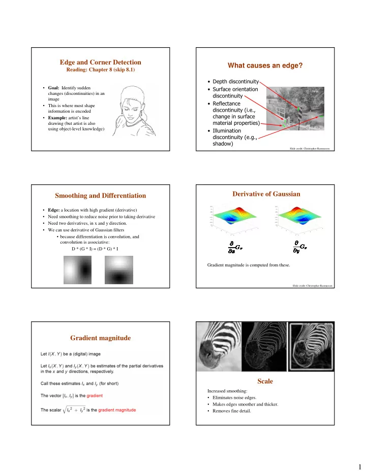
Edge and Corner Detection

Reading: Chapter 8 (skip 8.1)

• Goal: Identify sudden

changes (discontinuities) in an image

• This is where most shape

information is encoded

• Example: artist’s line

drawing (but artist is also using object-level knowledge)

What causes an edge?

• Slide credit: Christopher Rasmussen

Smoothing and Differentiation

• Edge: a location with high gradient (derivative)
• Need smoothing to reduce noise prior to taking derivative
• Need two derivatives, in x and y direction.
• We can use derivative of Gaussian filters
• because differentiation is convolution, and

convolution is associative: D * (G * I) = (D * G) * I

Derivative of Gaussian

Slide credit: Christopher Rasmussen

Gradient magnitude is computed from these.

Gradient magnitude Scale

Increased smoothing:

• Eliminates noise edges.
• Makes edges smoother and thicker.
• Removes fine detail.

2

Canny Edge Detection

Steps:

• 1. Apply derivative of Gaussian
• 2. Non-maximum suppression
• Thin multi-pixel wide “ridges” down to single

pixel width

• 3. Linking and thresholding
• Low, high edge-strength thresholds
• Accept all edges over low threshold that are

connected to edge over high threshold

• Matlab: edge(I, ‘canny’)

Non-maximum suppression: Select the single maximum point across the width

• f an edge.

Non-maximum suppression At q, the value must be larger than values interpolated at p or r.

Examples: Non-Maximum Suppression

• !"#
• Slide credit: Christopher Rasmussen

fine scale (σ = 1) high threshold

3

coarse scale, (σ = 4) high threshold coarse scale (σ = 4) low threshold

Linking to the next edge point

Assume the marked point is an edge point. Take the normal to the gradient at that point and use this to predict continuation points (either r or s).

Edge Hysteresis

• Hysteresis: A lag or momentum factor
• Idea: Maintain two thresholds khigh and klow

– Use khigh to find strong edges to start edge chain – Use klow to find weak edges which continue edge chain

• Typical ratio of thresholds is roughly

khigh / klow = 2

Example: Canny Edge Detection

• $
• %

&%

• Example:

Canny Edge Detection

'()

Slide credit: Christopher Rasmussen

4

Finding Corners

Edge detectors perform poorly at corners. Corners provide repeatable points for matching, so are worth detecting. Idea:

• Exactly at a corner, gradient is ill defined.
• However, in the region around a corner,

gradient has two or more different values.

The Harris corner detector

        =

∑ ∑ ∑ ∑

2 2 y y x y x x

I I I I I I C

Form the second-moment matrix:

Sum over a small region around the hypothetical corner Gradient with respect to x, times gradient with respect to y Matrix is symmetric

Slide credit: David Jacobs

      =         =

∑ ∑ ∑ ∑

2 1 2 2

λ λ

y y x y x x

I I I I I I C

First, consider case where: This means dominant gradient directions align with x or y axis If either λ is close to 0, then this is not a corner, so look for locations where both are large.

Simple Case

Slide credit: David Jacobs

General Case

It can be shown that since C is symmetric:

R R C       =

− 2 1 1

λ λ

So every case is like a rotated version of the

• ne on last slide.

Slide credit: David Jacobs

So, to detect corners

• Filter image with Gaussian to reduce noise
• Compute magnitude of the x and y gradients at

each pixel

• Construct C in a window around each pixel

(Harris uses a Gaussian window – just blur)

• Solve for product of λs (determinant of C)
• If λs are both big (product reaches local maximum

and is above threshold), we have a corner (Harris also checks that ratio of λs is not too high)

Gradient orientations

5

Closeup of gradient orientation at each pixel Corners are detected where the product of the ellipse axis lengths reaches a local maximum.

Harris corners

• Originally developed as features for motion tracking
• Greatly reduces amount of computation compared to

tracking every pixel

• Translation and rotation invariant (but not scale invariant)