
SLIDE 1
Hidden Markov Models DepmixS4 Examples Conclusions
depmixS4: an R-package for hidden Markov models
Ingmar Visser1 & Maarten Speekenbrink2
1Department of Psychology
University of Amsterdam
2Department of Psychology
University College London
Psychometric Computing, February 2011, Tuebingen
depmix Hidden Markov Models DepmixS4 Examples Conclusions
Outline
Hidden Markov Models DepmixS4 Examples Speed-accuracy trade-off Dynamic Change Card Sorting
depmix Hidden Markov Models DepmixS4 Examples Conclusions
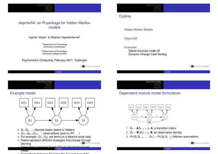
Example model
S1 S2 O11 O21 S3 O12 O22 O13 O23
◮ S1, S2, . . .: discrete states (latent or hidden) ◮ O11, O21, O12, . . .: observations (yes/no, RT, . . . ) ◮ For example: O11, O21 are items on a balance scale task ◮ States represent different strategies that change through
learning
◮ Dependency between S and O forms the measurement
model
◮ Dependency between S’s forms the dynamic part of the
depmix Hidden Markov Models DepmixS4 Examples Conclusions
Dependent mixture model formulation
S1 S2 O11 O21 S3 O12 O22 O13 O23
A A B B B B B B
- 1. St = ASt−1 + ξt, A, a transition matrix
- 2. Ot = B(St) + ζt, B, an observation density
- 3. Pr(St|St−1, . . . , S1) = Pr(St|St−1) (Markov assumption)
depmix