Outline Sequential Data - Part 2 Greg Mori - CMPT 419/726 Hidden - PDF document

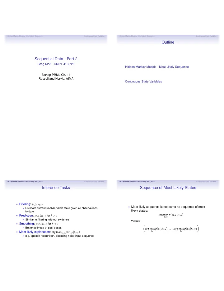
Hidden Markov Models - Most Likely Sequence Continuous State Variables Hidden Markov Models - Most Likely Sequence Continuous State Variables Outline Sequential Data - Part 2 Greg Mori - CMPT 419/726 Hidden Markov Models - Most Likely Sequence Bishop PRML Ch. 13 Russell and Norvig, AIMA Continuous State Variables Hidden Markov Models - Most Likely Sequence Continuous State Variables Hidden Markov Models - Most Likely Sequence Continuous State Variables Inference Tasks Sequence of Most Likely States • Filtering: p ( z t | x 1 : t ) • Most likely sequence is not same as sequence of most • Estimate current unobservable state given all observations likely states: to date arg max z 1 : N p ( z 1 : N | x 1 : N ) • Prediction: p ( z k | x 1 : t ) for k > t • Similar to filtering, without evidence versus • Smoothing: p ( z k | x 1 : t ) for k < t � � • Better estimate of past states z 1 p ( z 1 | x 1 : N ) , . . . , arg max z N p ( z N | x 1 : N ) arg max • Most likely explanation: arg max z 1 : N p ( z 1 : N | x 1 : N ) • e.g. speech recognition, decoding noisy input sequence

Hidden Markov Models - Most Likely Sequence Continuous State Variables Hidden Markov Models - Most Likely Sequence Continuous State Variables Paths Through HMM Viterbi Algorithm k = 1 k = 1 k = 2 k = 2 k = 3 k = 3 n − 2 n − 1 n n + 1 n − 2 n − 1 n n + 1 • Insight: for any value k for z n , the best path • There are K N paths to consider through the HMM for ( z 1 , z 2 , . . . , z n = k ) ending in z n = k consists of the best path computing ( z 1 , z 2 , . . . , z n − 1 = j ) for some j , plus one more step z 1 : N p ( z 1 : N | x 1 : N ) arg max • Don’t need to consider exponentially many paths, just K at each time step • Need a faster method • Dynamic programming algorithm – Viterbi algorithm Hidden Markov Models - Most Likely Sequence Continuous State Variables Hidden Markov Models - Most Likely Sequence Continuous State Variables Viterbi Algorithm - Math Viterbi Algorithm - Example Rain 1 Rain 2 Rain 3 Rain 4 Rain 5 k = 1 true true true true true state space paths k = 2 false false false false false true true false true true umbrella k = 3 .8182 .5155 .0361 .0334 .0210 n − 2 n − 1 n n + 1 most likely • Define message paths .1818 .0491 .1237 .0173 .0024 w ( n , k ) = max z 1 ,..., z n − 1 p ( x 1 , . . . , x n , z 1 , . . . , z n = k ) R t − 1 P ( R t ) R t P ( U t ) • From factorization of joint distribution: t 0.7 t 0.9 f 0.3 f 0.2 p ( rain 1 = true ) = 0 . 5 w ( n , k ) = z 1 ,..., z n − 1 p ( x 1 , . . . , x n − 1 , z 1 , . . . , z n − 1 ) p ( x n | z n = k ) p ( z n = k | z n − 1 ) max z 1 ,..., z n − 2 p ( x 1 : n − 1 , z 1 : n − 1 ) p ( x n | z n = k ) p ( z n = k | z n − 1 ) = max max w ( n , k ) = z 1 ,..., z n − 1 p ( x 1 , . . . , x n , z 1 , . . . , z n = k ) max z n − 1 w ( n − 1 , j ) p ( x n | z n = k ) p ( z n = k | z n − 1 = j ) = max = w ( n − 1 , j ) p ( x n | z n = k ) p ( z n = k | z n − 1 = j ) max j j

Hidden Markov Models - Most Likely Sequence Continuous State Variables Hidden Markov Models - Most Likely Sequence Continuous State Variables Viterbi Algorithm - Complexity Continuous State Variables z n − 1 z n +1 z 1 z 2 z n x 1 x 2 x n − 1 x n x n +1 • Each step of the algorithm takes O ( K 2 ) work • With N time steps, O ( NK 2 ) complexity to find most likely • In HMMs, the state variable z t is assumed discrete sequence • In many applications, z t is continuous • Much better than naive algorithm evaluating all K N possible • Object tracking paths • Stock price, gross domestic product (GDP) • Amount of rain • Can either discretize • Large state space • Discretization errors • Or use method that directly handles continuous variables Hidden Markov Models - Most Likely Sequence Continuous State Variables Hidden Markov Models - Most Likely Sequence Continuous State Variables Gaussianity Continuous State Variables - Filtering z n − 1 z n +1 z 1 z 2 z n • Recall the filtering problem p ( z t | x 1 : t ) distribution on current x 1 x 2 x n − 1 x n x n +1 state given all observations to date • As in discrete case, can formulate a recursive computation: • As in the HMM, we require model parameters – transition � p ( z t + 1 | x 1 : t + 1 ) = α p ( x t + 1 | z t + 1 ) p ( z t + 1 | z t ) p ( z t | x 1 : t ) model and sensor model z t • Unlike HMM, each of these is a conditional probability • Now we have an integral instead of a sum density given a continuous-valued z t • Can we do this integral exactly? • One common assumption is to let both be linear • If we use linear Gaussians, yes: Kalman filter Gaussians: • In general, no: can use particle filter p ( z t | z t − 1 ) = N ( z t ; Az t − 1 , Σ z ) p ( x t | z t ) = N ( x t ; Cz t , Σ x )

Hidden Markov Models - Most Likely Sequence Continuous State Variables Hidden Markov Models - Most Likely Sequence Continuous State Variables Particle Filter Recall: SIR - Algorithm • Sampling-importance-resampling algorithm has two stages • Sampling: • Draw samples z ( 1 ) , . . . , z ( L ) from proposal distribution q ( z ) • Importance resampling: • Put weights on samples p ( z ( l ) ) / q ( z ( l ) ) ˜ • The particle filter is a particular w l = � m ˜ p ( z ( m ) ) / q ( z ( m ) ) sampling-importance-resampling algorithm for z ( ℓ ) from the discrete set z ( 1 ) , . . . , z ( L ) • Draw samples ˆ approximating p ( z t | x 1 : t ) according to weights w l • Approximate p ( · ) by: L 1 � z ( ℓ ) ) p ( z ) ≈ δ ( z − ˆ L ℓ = 1 L � w ℓ δ ( z − z ( ℓ ) ) p ( z ) ≈ ℓ = 1 Hidden Markov Models - Most Likely Sequence Continuous State Variables Hidden Markov Models - Most Likely Sequence Continuous State Variables Particle Filter Particle Filter Illustration • The particle filter is a particular sampling- importance-resampling algorithm for approximating p ( z t | x 1 : t ) p ( z n | X n ) • What should be the proposal distribution q ( z t ) ? • Trick: use prediction given previous observations p ( z n +1 | X n ) L t − 1 p ( z t | z ( ℓ ) � w ℓ p ( z t | x 1 : t − 1 ) ≈ t − 1 ) ℓ = 1 p ( x n +1 | z n +1 ) • With this proposal distribution, the weights for importance resampling are: p ( z n +1 | X n +1 ) z p ( z ( ℓ ) p ( z ( ℓ ) ) | x 1 : t ) ˜ t w ℓ = q ( z ( ℓ ) ) = t p ( z ( ℓ ) | x 1 : t − 1 ) t p ( x t | z ( ℓ ) = ) t

Hidden Markov Models - Most Likely Sequence Continuous State Variables Hidden Markov Models - Most Likely Sequence Continuous State Variables Particle Filter Example Conclusion • Readings: Ch. 13.2.5, 13.3 • Most likely sequence in HMM • Viterbi algorithm – O ( NK 2 ) time, dynamic programming algorithm • Continuous state spaces • Linear Gaussians – closed-form filtering (and smoothing) using Kalman filter • General case – no closed-form solution, can use particle filter, a sampling method Okuma et al. ECCV 2004