
SLIDE 1
A spectral algorithm for learning hidden Markov models
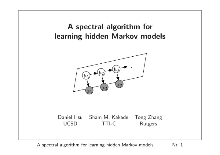
h1 x1 x2 h3 x3 . . . h2 Daniel Hsu Sham M. Kakade Tong Zhang UCSD TTI-C Rutgers
A spectral algorithm for learning hidden Markov models
- Nr. 1
A spectral algorithm for learning hidden Markov models . . . h 3 h - - PowerPoint PPT Presentation
A spectral algorithm for learning hidden Markov models . . . h 3 h 2 h 1 x 3 x 2 x 1 Daniel Hsu Sham M. Kakade Tong Zhang UCSD TTI-C Rutgers A spectral algorithm for learning hidden Markov models Nr. 1 Motivation Hidden Markov Models
h1
h2
ht+1
x1:t
△
h1
h2
h3
mAx2Ax1
R(U) = R(O)
△
mAxt . . . Ax1
m(U ⊤O)−1Bxt . . . Bx1(U ⊤O)
O T
Axt∼Bxt
U ⊤(O ht) Bxt(U ⊤O ht) = U ⊤(OAxt ht)
△
△
△
2,1
△
∞
△
∞
△
∞
v: v1=1 O