the central curve in linear programming
play

The Central Curve in Linear Programming Cynthia Vinzant, U. Michigan - PowerPoint PPT Presentation

The Central Curve in Linear Programming Cynthia Vinzant, U. Michigan joint work with Jes us De Loera and Bernd Sturmfels Cynthia Vinzant, U. Michigan The Central Curve in Linear Programming The Central Path of a Linear Program Linear


  1. The Central Curve in Linear Programming 
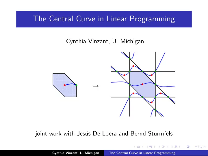
Cynthia Vinzant, U. Michigan → joint work with Jes´ us De Loera and Bernd Sturmfels Cynthia Vinzant, U. Michigan The Central Curve in Linear Programming

  2. The Central Path of a Linear Program Linear Program: Maximize x ∈ R n c · x s.t. A · x = b and x ≥ 0 . Cynthia Vinzant, U. Michigan The Central Curve in Linear Programming

  3. The Central Path of a Linear Program Linear Program: Maximize x ∈ R n c · x s.t. A · x = b and x ≥ 0 . Replace by : Maximize x ∈ R n f λ ( x ) s.t. A · x = b , where λ ∈ R + and f λ ( x ) := c · x + λ � n i =1 log | x i | . Cynthia Vinzant, U. Michigan The Central Curve in Linear Programming

  4. The Central Path of a Linear Program Linear Program: Maximize x ∈ R n c · x s.t. A · x = b and x ≥ 0 . Replace by : Maximize x ∈ R n f λ ( x ) s.t. A · x = b , where λ ∈ R + and f λ ( x ) := c · x + λ � n i =1 log | x i | . The maximum of the function f λ is attained by a unique point x ∗ ( λ ) in the the open polytope { x ∈ ( R > 0 ) n : A · x = b } . Cynthia Vinzant, U. Michigan The Central Curve in Linear Programming

  5. The Central Path of a Linear Program Linear Program: Maximize x ∈ R n c · x s.t. A · x = b and x ≥ 0 . Replace by : Maximize x ∈ R n f λ ( x ) s.t. A · x = b , where λ ∈ R + and f λ ( x ) := c · x + λ � n i =1 log | x i | . The maximum of the function f λ is attained by a unique point x ∗ ( λ ) in the the open polytope { x ∈ ( R > 0 ) n : A · x = b } . The central path is { x ∗ ( λ ) : λ > 0 } . As λ → 0 , the path leads from the analytic center of the polytope, x ∗ ( ∞ ), to the optimal vertex, x ∗ (0). Cynthia Vinzant, U. Michigan The Central Curve in Linear Programming

  6. The Central Path of a Linear Program The central path is { x ∗ ( λ ) : λ > 0 } . As λ → 0 , the path leads from the analytic center of the polytope, x ∗ ( ∞ ), to the optimal vertex, x ∗ (0). Cynthia Vinzant, U. Michigan The Central Curve in Linear Programming

  7. The Central Path of a Linear Program The central path is { x ∗ ( λ ) : λ > 0 } . As λ → 0 , the path leads from the analytic center of the polytope, x ∗ ( ∞ ), to the optimal vertex, x ∗ (0). Interior point methods ≈ piecewise-linear approx. of this path Cynthia Vinzant, U. Michigan The Central Curve in Linear Programming

  8. The Central Path of a Linear Program The central path is { x ∗ ( λ ) : λ > 0 } . As λ → 0 , the path leads from the analytic center of the polytope, x ∗ ( ∞ ), to the optimal vertex, x ∗ (0). Interior point methods ≈ piecewise-linear approx. of this path Bounds on curvature of the path → bounds on # Newton steps Cynthia Vinzant, U. Michigan The Central Curve in Linear Programming

  9. The Central Path of a Linear Program The central path is { x ∗ ( λ ) : λ > 0 } . As λ → 0 , the path leads from the analytic center of the polytope, x ∗ ( ∞ ), to the optimal vertex, x ∗ (0). Interior point methods ≈ piecewise-linear approx. of this path Bounds on curvature of the path → bounds on # Newton steps We can use concepts from algebraic geometry and matroid theory to bound the total curvature of the central path. Cynthia Vinzant, U. Michigan The Central Curve in Linear Programming

  10. The Central Curve The central curve C is the Zariski closure of the central path. It contains the central paths of all polyhedra in the hyperplane arrangement { x i = 0 } i =1 ,..., n ⊂ { A · x = b } . − → Zariski closure Cynthia Vinzant, U. Michigan The Central Curve in Linear Programming

  11. The Central Curve The central curve C is the Zariski closure of the central path. It contains the central paths of all polyhedra in the hyperplane arrangement { x i = 0 } i =1 ,..., n ⊂ { A · x = b } . − → Zariski closure Goal: Study the nice algebraic geometry of this curve and its applications to the linear program Cynthia Vinzant, U. Michigan The Central Curve in Linear Programming

  12. History and Contributions Motivating Question: What is the maximum total curvature of the central path given the size of the matrix A ? Cynthia Vinzant, U. Michigan The Central Curve in Linear Programming

  13. History and Contributions Motivating Question: What is the maximum total curvature of the central path given the size of the matrix A ? Deza-Terlaky-Zinchenko (2008) make continuous Hirsch conjecture Conjecture: The total curvature of the central path is at most O ( n ). Cynthia Vinzant, U. Michigan The Central Curve in Linear Programming

  14. History and Contributions Motivating Question: What is the maximum total curvature of the central path given the size of the matrix A ? Deza-Terlaky-Zinchenko (2008) make continuous Hirsch conjecture Conjecture: The total curvature of the central path is at most O ( n ). Dedieu-Malajovich-Shub (2005) apply differential and algebraic geometry to bound the total curvature of the central path. Cynthia Vinzant, U. Michigan The Central Curve in Linear Programming

  15. History and Contributions Motivating Question: What is the maximum total curvature of the central path given the size of the matrix A ? Deza-Terlaky-Zinchenko (2008) make continuous Hirsch conjecture Conjecture: The total curvature of the central path is at most O ( n ). Dedieu-Malajovich-Shub (2005) apply differential and algebraic geometry to bound the total curvature of the central path. Bayer-Lagarias (1989) study the central path as an algebraic object and suggest the problem of identifying its defining equations. Cynthia Vinzant, U. Michigan The Central Curve in Linear Programming

  16. History and Contributions Motivating Question: What is the maximum total curvature of the central path given the size of the matrix A ? Deza-Terlaky-Zinchenko (2008) make continuous Hirsch conjecture Conjecture: The total curvature of the central path is at most O ( n ). Dedieu-Malajovich-Shub (2005) apply differential and algebraic geometry to bound the total curvature of the central path. Bayer-Lagarias (1989) study the central path as an algebraic object and suggest the problem of identifying its defining equations. Our contribution is to use results from algebraic geometry and matroid theory to find defining equations of the central curve and refine bounds on its degree and total curvature. Cynthia Vinzant, U. Michigan The Central Curve in Linear Programming

  17. Outline ◦ Algebraic conditions for optimality ◦ Degree of the curve (and other combinatorial data) ◦ Total curvature and the Gauss map ◦ Defining equations ◦ The primal-dual picture Cynthia Vinzant, U. Michigan The Central Curve in Linear Programming

  18. Some details Here we assume that . . . 1) A is a d × n matrix of rank- d (possibly very special), and 2) c ∈ R n and b ∈ R d are generic. (This ensures that the central curve is irreducible and nonsingular.) Cynthia Vinzant, U. Michigan The Central Curve in Linear Programming

  19. Algebraic Conditions for Optimality . . . of the function f λ ( x ) = c · x + λ � n i =1 log | x i | in { A · x = b } : Cynthia Vinzant, U. Michigan The Central Curve in Linear Programming

  20. Algebraic Conditions for Optimality . . . of the function f λ ( x ) = c · x + λ � n i =1 log | x i | in { A · x = b } : c + λ x − 1 ∈ span { rows( A ) } ∇ f λ ( x ) = Cynthia Vinzant, U. Michigan The Central Curve in Linear Programming

  21. Algebraic Conditions for Optimality . . . of the function f λ ( x ) = c · x + λ � n i =1 log | x i | in { A · x = b } : c + λ x − 1 ∈ span { rows( A ) } ∇ f λ ( x ) = x − 1 ∈ span { rows( A ) } + λ − 1 c ⇒ Cynthia Vinzant, U. Michigan The Central Curve in Linear Programming

  22. Algebraic Conditions for Optimality . . . of the function f λ ( x ) = c · x + λ � n i =1 log | x i | in { A · x = b } : c + λ x − 1 ∈ span { rows( A ) } ∇ f λ ( x ) = x − 1 ∈ span { rows( A ) } + λ − 1 c ⇒ x − 1 ∈ span { rows( A ) , c } ⇒ Cynthia Vinzant, U. Michigan The Central Curve in Linear Programming

  23. Algebraic Conditions for Optimality . . . of the function f λ ( x ) = c · x + λ � n i =1 log | x i | in { A · x = b } : c + λ x − 1 ∈ span { rows( A ) } ∇ f λ ( x ) = x − 1 ∈ span { rows( A ) } + λ − 1 c ⇒ x − 1 ∈ span { rows( A ) , c } =: L A , c ⇒ Cynthia Vinzant, U. Michigan The Central Curve in Linear Programming

  24. Algebraic Conditions for Optimality . . . of the function f λ ( x ) = c · x + λ � n i =1 log | x i | in { A · x = b } : c + λ x − 1 ∈ span { rows( A ) } ∇ f λ ( x ) = x − 1 ∈ span { rows( A ) } + λ − 1 c ⇒ x − 1 ∈ span { rows( A ) , c } =: L A , c ⇒ L − 1 ⇒ x ∈ A , c where L − 1 A , c denotes the coordinate-wise reciprocal L A , c : � � L − 1 ( u − 1 1 , . . . , u − 1 A , c := n ) where ( u 1 , . . . , u n ) ∈ L A , c Cynthia Vinzant, U. Michigan The Central Curve in Linear Programming

Download Presentation
Download Policy: The content available on the website is offered to you 'AS IS' for your personal information and use only. It cannot be commercialized, licensed, or distributed on other websites without prior consent from the author. To download a presentation, simply click this link. If you encounter any difficulties during the download process, it's possible that the publisher has removed the file from their server.

Recommend


More recommend