Teaching Texture Mapping as a rectangular solid, and the lawn and - - PDF document

Teaching Texture Mapping Visually

Rosalee Wolfe DePaul University wolfe@cs.depaul.edu Visually demonstrating the behavior of texture mapping is beneficial to both computer science and art students. For computer science students it can serve as prelude to delving into the mathematical underpinnings of the topic, while in an art class it can be the main vehicle of explanation for students learning to use a rendering package as a medium of creative expression. The SIGGRAPH 97 Education Slide set covers not only the techniques of two- and three-dimensional texture mapping, but procedural textures, bump mapping, and environment mapping as well. In addition it discusses aliasing in texture mapping, and what can be done to counteract it. The following is a reprint of an article that appeared in the November 1997 issue of Computer Grapics and contains thumbnails and accompanying narrative for the slide set. To order the full color 35mm slide set, call ACM Member Services at 800 342 6626 in the U.S. and Canada, and +1 212 626 0500 for the greater New York area and all other countries. The ACM order number of the education slide set is 434975 (ISBN 0 89791 956-4) and the price is $35.00 for ACM/ SIGGRAPH members and $45 for non- members.

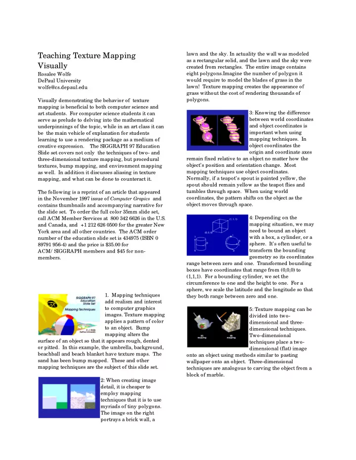
• 1. Mapping techniques

add realism and interest to computer graphics

• images. Texture mapping

applies a pattern of color to an object. Bump mapping alters the surface of an object so that it appears rough, dented

• r pitted. In this example, the umbrella, background,

beachball and beach blanket have texture maps. The sand has been bump mapped. These and other mapping techniques are the subject of this slide set. 2: When creating image detail, it is cheaper to employ mapping techniques that it is to use myriads of tiny polygons. The image on the right portrays a brick wall, a lawn and the sky. In actuality the wall was modeled as a rectangular solid, and the lawn and the sky were created from rectangles. The entire image contains eight polygons.Imagine the number of polygon it would require to model the blades of grass in the lawn! Texture mapping creates the appearance of grass without the cost of rendering thousands of polygons. 3: Knowing the difference between world coordinates and object coordinates is important when using mapping techniques. In

• bject coordinates the
• rigin and coordinate axes

remain fixed relative to an object no matter how the

• bject’s position and orientation change. Most

mapping techniques use object coordinates. Normally, if a teapot’s spout is painted yellow, the spout should remain yellow as the teapot flies and tumbles through space. When using world coordinates, the pattern shifts on the object as the

• bject moves through space.

4: Depending on the mapping situation, we may need to bound an object with a box, a cylinder, or a

• sphere. It’s often useful to

transform the bounding geometry so its coordinates range between zero and one. Transformed bounding boxes have coordinates that range from (0,0,0) to (1,1,1). For a bounding cylinder, we set the circumference to one and the height to one. For a sphere, we scale the latitude and the longitude so that they both range between zero and one. 5: Texture mapping can be divided into two- dimensional and three- dimensional techniques. Two-dimensional techniques place a two- dimensional (flat) image

• nto an object using methods similar to pasting

wallpaper onto an object. Three-dimensional techniques are analogous to carving the object from a block of marble.

2

6: Two-dimensional mappings use pre- existing images. This slide shows some images that might be used for texture mapping. The images on the left are either scanned photographs or images created in a paint or drawing package. POVRay, a raytracer, created the images on the right. 7: In two-dimensional texture mapping, we have to decide how to paste the image on to an

• bject. In other words,

for each pixel in an

• bject, we encounter the

question, “ Where do I have to look in the texture map to find the color?” To answer this question, we consider two things: map shape and map entity. 8: We’ll discuss map shapes first. For a map shape that’s planar, we take an (x,y,z) value from the object and throw away (project) one of the components, which leaves us with a two-dimensional (planar) coordinate. We use the planar coordinate to look up the color in the texture map. 9: This slide shows several textured-mapped

• bjects that have a planar

map shape. None of the

• bjects have been rotated.

In this case, the component that was thrown away was the z-coordinate. You can determine which component was projected by looking for color changes in coordinate directions. When moving parallel to the x-axis, an object’s color

• changes. When moving up and down along the y-

axis, the object’s color also changes. However, movement along the z-axis does not produce a change in color. This is how you can tell that the z- component was eliminated. 10: In the left image, an

• bjects color changes

when there’s a change in y, or when there’s a change in z, but the color remains constant when x

• changes. Which

component was projected? In the right image, which component was projected? 11: A second shape used in texture mapping is a

• cylinder. An (x,y,z) value

is converted to cylindrical coordinates of (r, theta, height). For texture mapping, we are only interested in theta and the height. To find the color in two-dimensional texture map, theta is converted into an x-coordinate and height is converted into a y-

• coordinate. This wraps the two-dimensional texture

map around the object. 12: The texture-mapped

• bjects in this image have

a cylindrical map shape, and the cylinder’s axis is parallel to the z-axis. At the smallest z-position on each object, note that the squares of the texture pattern become squeezed into “ pie slices” . This phenomenon occurs at the greatest z position as well. When the cylinder’s axis is parallel to the z-axis, you’ll see “ pie slices” radiating out along the x- and y- axes. 13:On the left squares of the texture map are squeezed into pie slices that radiate out along the x- and z-axes. Which coordinate axis is parallel to the cylinder’s axis? 14: When using a sphere as the map shape, the (x,y,z) value of a point is converted into spherical

• coordinates. For

purposes of texture mapping, we keep just the latitude and the longitude information. To find the color in the texture map, the latitude is converted into an x-coordinate and the longitude is converted into a y-coordinate.

3

15: The objects have a map shape of a sphere, and the poles of the sphere are parallel to the y-axis. At the object’s “ North Pole” and “ South Pole” , the squares of the texture map become squeezed into pie-wedge shapes. Compare this slide to slide 12 which has a map shape

• f a cylinder. Both map shapes have the pie-wedge

shapes at the poles, but there is a subtle difference at the object’s “ equator” . The spherical mapping stretches the squares in the texture map near the equator, and squeezes the squares as the longitude reaches a pole. 16: These objects have a spherical map shape. 17: Using a box as the map shape is similar to planar mapping. Instead

• f using one texture map,

box mapping uses six --

• ne each for the left,

right, front, back, top and bottom sides of the object. To texture map the front and back sides, we eliminate the z-component of an

• bject’s point and use the remaining x- and y-

components to locate the color in the corresponding texture maps. 18: Here are six textures that we will use in our next example. 19: The objects in slide have a box as the map shape. 20: Here’s another six

• textures. This scene was

modeled by Steve van der Burg. 21: Here’s the result. 22: Remember that we choose a map shape and a map entity when texture mapping. When discussing map shape, we talked about taking an (x,y,z) value from the object and converting in various ways, but we didn’t mention what that value was. The map entity determines what we use as the (x,y,z) value. Commonly-used map entities are 1) a point on the

• bject relative to the object’s bounding box, 2) the

surface normal at the point being rendered, 3) a vector running from the object’s centroid through the point, and 4) the reflection vector at the current point. Remember that the reflection vector depends not only

• n the position of the point and its normal, but on the

position of the viewer. 23: This next sequence of slides shows the interaction of map shape and map parameter. The map shape is the same for all the teapots on this

• slide. What is it?

24: Some combinations of map shape and map parameter produce more useful results than others. For a cylindrical map shape, which map parameters seem to produce the best results?

4

25: Which map parameters look good with a spherical map shape? Compare map parameters best for cylindrical map shape with those best for a spherical map shape. Are there any similarities? 26: Can you guess the map shape? 27: When rendering a parametric patch, we can dispense with map shape and map entity by treating the u- and v- parameters of the surface as if they were normalized device coordinates (Catmull, 1974). Multiplying u and v by the resolution (in pixels) yields the device coordinates of the desired pixel in the texture map. 28: Here is the same patch with its texture map. 29: The model for this teapot has 32 parametric patches, each of which sports a copy of the

• texture. This slide shows

the use of the u,v parameters to select the coordinates of desired color in the texture image. 30: This technique can be applied to objects that aren’t parametrically defined by assigning u,v values to each vertex. As long as the chosen values range between zero and

• ne, it’s possible to use the same texture mapping

approach. 31: By using a nonlinear function, it’s possible to pull or distort the texture maps over the surface of polygons. 32: We can layer textures

• ne on top of another by

using a technique similar to the one that allows television viewers to see a forecaster standing in front of a weather map when in actuality the forecaster is standing in front of a blue wall in a studio. The colors of the background weather map is substituted for the blue color. (Have you noticed that they never wear blue?) We can do the same thing. We want to place the word “ hello”

• n top of a map of the world. The black background
• f the “ hello” image will be treated as transparent. To

create a pixel in the final image, we find the colors in the corresponding pixel locations in the two input images and combine the two. 33: Here is an example of layered textures. :-)

• 34. Bo Peep is a character from “ Toy Story” . “ Toy

Story” made history as the first computer animated feature film and was created by Disney and Pixar. What texture techniques are at work in this image? What was the map shape for the wall? For the lamp? 35: A major drawback to 2D texture mapping is the necessity of handling

• singularities. For

instance, a spherical mapping has two singularities, one each at the North and South

• Poles. J

ust as it makes no sense to talk about the time zone at the North Pole, it’s impossible to determine the second texture coordinate by the usual mathematical conversion. A programmer has to

5

anticipate singularities and handle them as special cases or the program will bomb. 36: In a 2D planar mapping, a checker pattern degenerates into stripes along the axis being projected, which does not happen with a 3D mapping of a checker pattern. 37: In three-dimensional texture mapping, each point determines its color without the use of an intermediate map shape (Peachey, 1985; Perlin, 1985). We use the (x,y,z) coordinate to compute the color directly. It’s equivalent to carving an object out of a solid

• substance. Most 3D texture functions do not

explicitly store a value for each (x, y, z)-coordinate, but use a procedure to compute a value based on the coordinate and thus are called procedural textures. 38: To put stripes the left teapot, we find the integer part of the z-value

• f each point of the
• bject. If resulting value

is even, we choose red;

• therwise we choose
• white. How were the stripes produced in the other

two teapots? 39: To produce the rings in the upper left teapot, we use the x- and y- components to compute the distance of a point from the object’s center, and truncate the result. If the resulting value is even, we choose red; otherwise we choose white. Which two components were used to produce the rings on the upper right teapot? 40: Here are textures created by ramp and sine

• functions. A nice ramp is

created by the function mod(x,a)/

• a. This ramp

function has a range of zero to one, as does (sin(x)+1)/

• 2. In this picture, we assigned magenta to

value of zero and yellow to the value one. Which of these teapot is using a sine function? How do you know? 41: We can use a point to compute an index into a color table. One way to do this is to keep the fractional part of the x- coordinate, which ranges between zero and one, and multiply it by the number of elements in the color table. 42: Regular patterns are not as interesting as patterns with some

• randomness. For texture

mapping the randomness is produced by a noise

• function. Desirable

properties for such a noise function are (Perlin, 1985): * known range * stationary * band limited * isotropic 43: Lattice noise has these desirable

• properties. It stores a

number from the random number generator at each integer lattice point in a 3D array. If a point from the object happens to have integer coordinates, a lattice noise function does a table lookup to find the value to return. If the object’s point has non-integer values, the function uses trilinear interpolation to determine the returned value. 44: A second technique for producing “ nice noise” is called gradient

• noise. Gradient noise

generates random unit vectors for each integer lattice point, and uses interpolation to find values for non-integer coordinates. 45: In lattice noise, maxima and minima always occur at regularly-spaced intervals, since it first fixes values to the (integer) positions of the

6

lattice and interpolates to obtain intermediate values. The regularity of these maxima and minima can be noticeable to an observer, as demonstrated in this

• slide. Gradient noise does not suffer from this

problem. 46: We can change the frequency and amplitude to vary the nature of the

• noise. The middle image

in this slide depicts the function noise(x,y,z) We can vary the effect of the noise by using the expression noise(f*x, f*y, f*z) * a where f controls the frequency and a controls the

• amplitude. Noise having large amplitudes will result

in a greater range of colors. Noise having high frequency will contain more detail. In the slide there are four images surrounding the depiction of the

• riginal noise function. Which image portrays noise

having lower frequency and lower amplitude than the

• riginal? Which has higher frequency and lower

amplitude? 47: This is a demonstration of how 1/ f noise is created. We begin with a noise function, depicted on the

• left. To this we add the

same noise function with twice the frequency and half the amplitude, which results in the second picture. The third image is the sum of the noise in the second picture plus the noise function with four times the frequency and a quarter

• f the amplitude. We can continue adding noise of

higher and higher frequency until the frequency is so high that something as large as a pixel won’t be able to record it. 48: Here we finally begin seeing some application

• f noise to texture
• mapping. To get a

Wisconsin-styled black- and-white spotted teapot, use the following pseudocode: gray = noise(x,y,z) if(gray > threshold) choose white else choose black 49: Perturbing stripes can result in a texture with a marbled appearance. 50: This is the “ Grateful Teapot” , created by perturbing a “ pinwheel texture” to produce an index into a color table. This texture was created by Kevin Ferguson. 51: Making a wood- grained object begins with a three-dimensional texture of concentric rings (Peachey, 1985). By using noise to vary the ring shape and the inter-ring distance, we can create reasonably realistic wood. 52: We can create an irridescence effect by combining the color from a color table with the

• bject’s original color.

Adding noise to perturb the color table lookup creates a mother-of-pearl effect. 53: Procedural functions can not only determine an

• bject’s color, but its

geometry as well. Volume density functions describe the geometry of gases and are similar to solid texturing procedures in that they take a point in three- dimensional space as input and return a value. Instead of returning a color, they return a density

• value. The cloud in this image is a procedurally

altered metaball created by David Ebert. 54: This still is from the movie “ Getting Into Art” , by David Ebert and diplays another example another example of a volume density function. Name the texture

7

mapping techniques you see. Which are the 3D textures? 55: All the frames in the movie “ Toy Story” were rendered using Pixar’s Photorealistic

• Renderman. In

Renderman, textures are added via the use of “ shaders” . Compare the horse pattern on the quilt to the wood pattern in the headboard. Which is more likely to be a 3D texture? 56: Bump mapping affects object surfaces, making them appear rough, wrinkled, or dented (Blinn, 1978). Bump mapping alters the surface normals before the shading calculation takes place. It’s possible to change a surface normals magnitude or direction. 57: In the upper left image, lattice noise alters the magnitude of the teapot’s surface normals, which creates a rough- looking surface. Lattice noise at a lower frequency changes the magnitude of the surface normals of the upper right teapot. It appears dented. The lower left teapot is the result of using sin(y)/ 2 + .5 to scale the normals magnitude, which results in a rippled effect. In all cases the profile of the teapot is still smooth. Bump mapping does not change the underlying geometry of the model, but fools the shading algorithm to produce an interesting surface. 58: In contast, displacement mapping alters an object’s geometry (Cook, 1984). Compare the profiles and the shadows cast by these two objects. Which is bump mapped? 59: Embossing is a form of bump mapping. To emboss the letter “ D” onto the teapot, we map each point of the object into the “ D” image. If we land at a location where there is a transition from white to black, then we rotate the point’s surface normal by an angle theta. If we land at a location in the “ D” where there is a transition from black to white, then we rotate the point’s surface normal by -theta. If we land at a location where there is no transition, we don’t do anything to the surface normal. 60: Environment mapping is a cheap way to create reflections (Blinn and Newell, 1976). While it’s easy to create reflections with a ray tracer, ray tracing is still too expensive for long animations. Adding an environment mapping feature to a z-buffer based renderer will create reflections that are acceptable in a lot of

• situations. Environment

mapping is a two- dimensional texture mapping technique that uses a map shape of a box and a map parameter of a reflection ray. 61: Here are side-by-side comparisons of raytracing and environment mapping. What differences can you see? 62: Environment mapping is cheaper than raytracing and works well when the reflective surface is planar or convex and there are no obvious sets of parallel lines in the

• reflection. In the top example the results from

environment mapping compare favorably with raytracing, but in the lower example, the reflected lines of the ceiling tiles do not align with the actual ceiling. 63: Notice the difference in rendering times between raytracing and environment mapping. Compare the difference in appearance.

8

64: In this still from “ Toy Story,” what techniques are being applied Slinky Dog’s ear and Rex’s skin? This image is not raytraced, yet reflections

• f Slinky Dog and Rex

are visible in the highly polished floor. What technique created this effect? 65: No matter the type of mapping we’re undertaking, we run the danger of

• aliasing. Aliasing can ruin the appearance of a

texture-mapped object. 66: Aliasing is caused by

• undersampling. Two

adjacent pixels in an

• bject may not map to

adjacent pixels in the texture map. As a result, some

• f the information from the texture map is lost when

it is applied to the object. 67: Antialiasing minimizes the effects of

• aliasing. One method,

called prefiltering, treats a pixel on the object as an area (Catmull, 1978). It maps the pixel’s area into the texture map. The average color is computed from the pixels inside the area swept out in the texture map. 68: A second method, called supersampling, also computes an average color (Crow, 1981). In this example each of four corners of an object pixel are mapped into the

• texture. The four pixels from the texture map are

averaged to produce the final color for the object. 69: Prefiltering in action 70: Supersampling in action. 71: Antialiasing is expensive due to the additional computation required to compute an average color. Mipmapping saves some expense by precalculating some average colors (Williams, 1983). The mipmap algorithm first creates several versions

• f the texture. Beginning with the original texture the

mipmap algorithm computes a new texture that’s one fourth the size. In the new, smaller texture map, each pixel contains the average of four pixels from the

• riginal texture. The process of creating smaller

images continues until we get a texture map containing one pixel. That one pixel contains the average color of the original texture map in its entirety. 72: In the texture mapping phase the area of each pixel on the object is mapped into the original texture map. The mipmap computes a measure of how many texture pixels are in the area defined by the mapped pixel. In this example approximately nine texture pixels will influence the final color so the ratio of texture pixels to object pixel is 9:1. 73: To compute the final color, we find the two texture maps whose ratios of texture pixels are closest to the ratio for the current object

• pixel. We look up the pixel colors in these two maps

and average them.

9

74: All images are rendered at 512x324. The upper left figure is not antialiased. The figure to its right was rendered with mipmapping. The textures are a little

• better. In the bottom row, the left image was

supersampled at a rate of nine samples to one pixel. The final image benefited from 9:1 supersampling and mipmapping. 75-79: The final series of slides, courtesy of Evans and Sutherland, demonstrate mipmapping. The foreground in these images is texture mapped using the bigger mipmaps containing more detail, with the smaller mipmaps reserved for the background. In slide 75, compare cultivated fields in the foreground with those in the background. The technique is effective in simulating a wide variety of terrains, as can be seen in slides 76-78. Evans and Sutherland develop flight simulators to train pilots. These simulators project views of what the pilot would see if actually flying the plane (slide 79). The simulators change the views as the pilot flies the plane, and must react instaneously with new views in response to pilot

• commands. Mipmapping heightens the sense of

reality by adding detail to the views. References (Blinn, 1978) J . Blinn, Simulations of Wrinkled

• Surfaces. Computer Graphics 12(3) August

1978, 286-292. (Blinn and Newell, 1976) J . Blinn and M. Newell, Texture and Reflection in Computer Generated Images. Communications of the ACM 19(10) October 1976, 542-546. (Catmull, 1974) E. Catmull, A Subdivision Algorithm for Computer Display of Curved Surfaces. PhD thesis, Department of Computer Science, University of Utah, December 1974. (Catmull, 1978) E. Catmull, A Hidden-Surface Algorithm with Anti-Aliasing. Computer Graphics 12 (3) August 1978, 6-10. (Cook, 1984) R. Cook, Shade Trees. Computer Graphics 18 (3) J uly 1984 223-231. (Crow, 1981) F. Crow, A Comparison of Antialiasing

• Techniques. IEEE Computer Graphics and
• Applications. 1 (1) J

anuary 1981, 40-49. (Peachey, 1985) D. Peachey, Solid Texturing of Complex Surfaces. Computer Graphics 19 (3) J uly 1985, 279-286. (Perlin, 1985) K. Perlin, An Image Synthesizer. Computer Graphics 19 (3) J uly 1985, 287-296. (Williams, 1983) L. Williams, Pyradmial Parametrics. Computer Graphics 17 (3) J uly 1983, 1-11. For more information on mapping techniques, see:

• D. Ebert, F. K. Musgrave, D. Peachey, K. Perlin and S.

Worley, Texturing and Modeling: A Procedural

• Approach. Academic Press, 1994.

J . Foley, A. vanDam, S. Feiner and J . Hughes, Computer Graphics: Principles and Practice.

• 2nd. ed. Addison-Wesley, 1990.
• A. Watt and M. Watt, Advanced Animation and

Rendering Techniques: Theory and Practice. Addison-Wesley, 1992. Credits The dining room seen in slides 6 and 22 was created by Steve van der Burg and rendered using POVRay. The teapots in slides 11 and 14 as well as the raytracing examples on slides 61-63 were done rendered using Craig Kolb’s Rayshade. David Ebert contributed slides 53 and 54. (Thanks, David!) The scene in slides 62 and 63 was created using Steven Chenney’s Sced. Kevin Ferguson developed the “ pinwheel texture” to create the Grateful Teapot in slide 50. Pixar and Disney graciously donated the “ Toy Story” images (slides 36, 55, and 64). Through Dave Tubbs, Evans and Sutherland generously donated slides 75-79. All other slides were created with custom rendering software developed at DePaul University. Textures for the beachball and towel in the title slide came from the SIGGRAPH 97 beachball and committee “ surfer” shirt. Many people contributed time, expertise and creativity to this slide set. Thanks to Steve Cunningham for initial discussions that formed the core material for set and for his patience in reviewing many, many drafts. Alain Chesnais made many substantive and constructive comments and suggested the slides on parametric mapping and the visual comparison of lattice and gradient noise. Stephen Spencer, J udy Brown and Tom Rieke also made excellent suggestions for improvement to both the images and the text. J ackie White was most gracious in lending her time, despite adverse condition, to help create the title slide. An extra thanks you goes to Stephen Spencer who as Director

10

for Publications supported the development of this set. Thanks also to the 1997 Graphics students at DePaul, especially Olivier Buisard, who class-tested these images.