Outline Texture Mapping Modeling surface details with images. - - PowerPoint PPT Presentation

Texture Mapping

Roger Crawfis Ohio State University

Outline

• Modeling surface details with images.
• Texture parameterization
• Texture evaluation
• Anti-aliasing and textures.

Texture Mapping

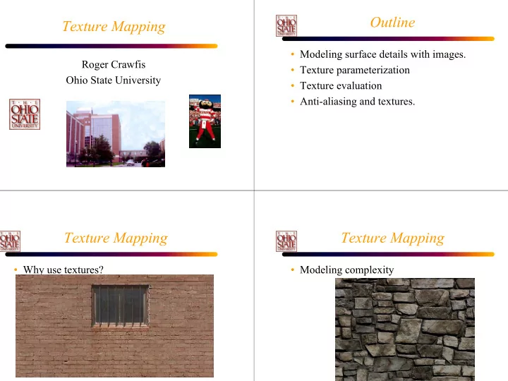
• Why use textures?

Texture Mapping

• Modeling complexity

Quote

“I am interested in the effects on an object that speak of human intervention. This is another factor that you must take into consideration. How many times has the object been painted? Written on? Treated? Bumped into? Scraped? This is when things get exciting. I am curious about: the wearing away of paint on steps from continual use; scrapes made by a moving dolly along the baseboard

• f a wall; acrylic paint peeling away from a previous coat
• f an oil base paint; cigarette burns on tile or wood floors;

chewing gum – the black spots on city sidewalks; lover’s names and initials scratched onto park benches…”

• Owen Demers

[digital] Texturing & Painting, 2002

Texture Mapping

• Given an object and an image:

– How does the image map to the vertices or set

• f points defining the object?

Jason Bryan

Texture Mapping

Jason Bryan

Texture Mapping

Jason Bryan

Texture Mapping

Jason Bryan

Texture Mapping

Jason Bryan

Texture Mapping

• Given an object and an image:

– How does the image map to the vertices or set

• f points defining the object?

Texture Mapping

• Given an object with an image mapped to it:

– How do we use the color information from the texture image to determine a pixel’s color?

Texture Mapping

• Problem #1 Fitting a square peg in a round

hole

Texture Mapping

• Problem #2 Mapping from a pixel to a texel

What is an image?

• How would I rotate an image 45 degrees?
• How would I translate it 0.5 pixels?

What is a Texture?

• Given the (u,v), want:

– – F F(u,v) ==> a continuous reconstruction

• = { R(u,v), G(u,v), B(u,v) }
• = { I(u,v) }
• = { index(u,v) }
• = { alpha(u,v) }
• = { normals(u,v) }
• = { surface_height(u,v) }
• = ...

What is the source of your Texture?

• Procedural Image
• RGB Image
• Intensity image
• Opacity table

Procedural Texture

Periodic and everything else

Checkerboard Scale: s= 10 If (u * s) % 2=0 && (v * s)%2=0 texture(u,v) = 0; // black Else texture(u,v) = 1; // white

RGB Textures

• Places an image on the object

Camuto 1998

Intensity Modulation Textures

• Multiply the objects color by that of the

texture.

Opacity Textures

• A binary mask, really redefines the

geometry.

Color Index Textures

• New Microsoft Extension for 8-bit textures.
• Also some cool new extensions to SGI’s

OpenGL to perform table look-ups after the texture samples have been computed.

Lao 1998

Bump Mapping

• This modifies the surface normals.
• More on this later.

Lao 1998

Displacement Mapping

• Modifies the surface position in the

direction of the surface normal.

Lao 1998

Reflection Properties

• Kd, Ks
• BDRF’s

– Brushed Aluminum – Tweed – Non-isotropic or anisotropic surface micro facets.

Texture and Texel

• Each pixel in a texture map is called a Texel
• Each Texel is associated with a 2D, (u,v),

texture coordinate

• The range of u, v is [0.0,1.0]

(u,v) tuple

• For any (u,v) in the range of (0-1, 0-1), we

can find the corresponding value in the texture using some interpolation

Two-Stage Mapping

• 1. Model the mapping: (x,y,z) -> (u,v)
• 2. Do the mapping

Image space scan

For each scanline, y

For each pixel, x compute u(x,y) and v(x,y) copy texture(u,v) to image(x,y)

• Samples the warped texture at the

appropriate image pixels.

• inverse mapping

Texture

Image space scan

• Problems:

– Finding the inverse mapping

• Use one of the analytical mappings that are

invertable.

• Bi-linear or triangle inverse mapping

– May miss parts of the texture map

Image

Texture space scan

For each v

For each u compute x(u,v) and y(u,v) copy texture(u,v) to image(x,y)

• Places each texture sample to the mapped

image pixel.

• forward mapping

Texture space scan

• Problems:

– May not fill image – Forward mapping needed

Image Texture

Continuous functions F(u,v)

• We are given a discrete set of values:

– F[i,j] for i=0,…,N, j=0,…,M

• Nearest neighbor:

– – F F(u,v) = F[ round(N*u), round(M*v) ]

• Linear Interpolation:

– i = floor(N*u), j = floor(M*v) – interpolate from F[i,j], F[i+1,j], F[i,j+1], F[i+1,j+1]

How do we get F(u,v)?

• Higher-order interpolation

– – F F(u,v) = ∑ i∑j F[i,j] h(u,v) – h(u,v) is called the reconstruction kernel

• Guassian
• Sinc function
• splines

– Like linear interpolation, need to find neighbors.

• Usually four to sixteen

Texture Parameterization

• Definition:

– The process of assigning texture coordinates or a texture mapping to an object.

• The mapping can be applied:

– Per-pixel – Per-vertex

Texture Parameterization

• Mapping to a 3D Plane

– Simple Affine transformation

• rotate
• scale
• translate

z y x u v

Texture Parameterization

• Mapping to a Cylinder

– Rotate, translate and scale in the uv-plane – u -> theta – v -> z – x = r cos(theta), y = r sin(theta)

u v

Texture Parameterization

• Mapping to Sphere

– Impossible!!!! – Severe distortion at the poles – u -> theta – v -> phi – x = r sin(theta) cos(phi) – y = r sin(theta) sin(phi) – z = r cos(theta)

Texture Parameterization

• Mapping to a Sphere

u v

Example (Rogers)

• Setup up surface, define correspondence, and voila!

x(θ,φ) = sin θ sin φ y(θ,φ) = cos φ z(θ,φ) = cos θ sin φ 0 ≤ θ ≤ π/2 π/4 ≤ φ ≤ π/2 Part of a sphere (u,v) = (0,0) ⇔ (θ,φ) = (0, π/2) (u,v) = (1,0) ⇔ (θ,φ) = (π/2, π/2) (u,v) = (0,1) ⇔ (θ,φ) = (0, π/4) (u,v) = (1,1) ⇔ (θ,φ) = (π/2, π/4)

Example Continued

• Can even solve for (θ,φ) and (u,v)

– A= π/2, B=0, C=-π/4, D=π/2

4 2 2

) , ( ) , ( 4 2 ) , ( 2 ) , (

π π π

φ φ θ θ φ θ π π φ π θ − = = − = = v u v v u u v u So looks like we have the texture space ⇔ object space part done!

All Is Not Good

• Let’s take a closer look:

Started with squares and ended with curves It only gets worse for larger parts of the sphere

Texture Parameterization

• Mapping to a Cube

u v common seam

Two-pass Mappings

• Map texture to:

– Plane – Cylinder – Sphere – Box

• Map object to same.

u v u-axis

S and O Mapping

• Pre-distort the texture by mapping it onto a

simple surface like a plane, cylinder, sphere,

• r box
• Map the result of that onto the surface
• Texture → Intermediate is S mapping
• Intermediate → Object is O mapping

(u,v) (xi,yi) (xo,yo,zo) S T Texture space Intermediate space Object space

S Mapping Example

• Cylindrical Mapping

A B A A B A

z z z z t s − − = − − = θ θ θ θ

O Mapping

• A method to relate the surface to the cylinder
• r
• r

O Mappings Cont’d

• Bier and Sloan defined 4 main ways

Reflected ray Object normal Object centroid Intermediate surface normal

Texture Parameterization

• Plane/ISN (projector)

– Works well for planar objects

• Cylinder/ISN (shrink-wrap)

– Works well for solids of revolution

• Box/ISN
• Sphere/Centroid
• Box/Centroid

Works well for roughly spherical shapes

Texture Parameterization

• Plane/ISN

Texture Parameterization

• Plane/ISN

– Resembles a slide projector – Distortions on surfaces perpendicular to the plane.

Watt

Texture Parameterization

• Plane/ISN

– Draw vector from point (vertex or object space pixel point) in the direction of the texture plane. – The vector will intersect the plane at some point depending on the coordinate system

Texture Parameterization

• Cylinder/ISN

– Distortions on horizontal planes – Draw vector from point to cylinder – Vector connects point to cylinder axis

Watt

Texture Parameterization

• Sphere/ISN

– Small distortion everywhere. – Draw vector from sphere center through point on the surface and intersect it with the sphere.

Watt

Texture Parameterization

• What is this ISN?

– Intermediate surface normal. – Needed to handle concave objects properly. – Sudden flip in texture coordinates when the

• bject crosses the axis.

Texture Parameterization

• Flip direction of

vector such that it points in the same half-space as the

• utward surface

normal.

Triangle Mapping

• Given: a triangle with texture coordinates at

each vertex.

• Find the texture coordinates at each point

within the triangle.

U=0,v=0 U=1,v=1 U=1,v=0

Triangle Mapping

• Given: a triangle with texture coordinates at

each vertex.

• Find the texture coordinates at each point

within the triangle.

U=0,v=0 U=0,v=1 U=1,v=0

Triangle Mapping

• Triangles define linear mappings.
• u(x,y,z) = Ax + By + Cz + D
• v(x,y,z) = Ex + Fy + Gz + H
• Plug in the each point and corresponding

texture coordinate.

• Three equations and three unknowns
• Need to handle special cases: u==u(x,y) or

v==v(x), etc.

Triangle Interpolation

• The equation: f(x,y) = Ax+By+C defines a linear

function in 2D.

• Knowing the values of f() at three

locations gives us enough information to solve for A, B and C.

• Provided the triangle

lies in the xy-plane.

Triangle Interpolation

• We need to find two 3D functions: u(x,y,z)

and v(x,y,z).

• However, there is a relationship between x,

y and z, so they are not independent.

• The plane equation of the triangle yields:

z = Ax + By + D

Triangle Interpolation

• A linear function in 3D is defined as

– f(x,y,z) = Ax + By + Cz + D

• Note, four points uniquely determine this

equation, hence a tetrahedron has a unique linear function through it.

• Taking a slice plane through this gives us a

linear function on the plane.

Triangle Interpolation

• Plugging in z from the plane equation.

f(x,y,z) = Ax + By + C(Ex+Fy+G) + D = A’x + B’y + D’

• For u, we are given:

C By Ax u C By Ax u C By Ax u + + = + + = + + =

2 2 2 1 1 1

Triangle Interpolation

• We get a similar set of equations for

v(x,y,z).

• Note, that if the points lie in a plane parallel

to the xz or yz-planes, then z is undefined.

• We should then solve the plane equation for

y or x, respectively.

• For robustness, solve the plane equation for

the term with the highest coefficient.

Quadrilateral Mapping

• Given: four texture coordinates on four

vertices of a quadrilateral.

• Determine the texture coordinates

throughout the quadrilateral.

Inverse Bilinear Interpolation

• Given a quadrilateral with texture

coordinates at each vertex

• The exact mapping, M, is unknown

u v x y z xs ys T-1 M-1 P0 P1 P2 P3

Inverse Bilinear Interpolation

• Given:

– (x0,y0,u0,v0) – (x1,y1,u1,v1) – (x2,y2,u2,v2) – (x3,y3,u3,v3) – (xs,ys,zs) - The screen coords. w/depth – T-1

• Calculate (xt,yt,zt) from T-1*(xs,ys,zs)

Inverse Bilinear Interpolation

Barycentric Coordinates: x(s,t) = x0(1-s)(1-t) + x1(s)(1-t) + x2(s)(t) + x3(1-s)(t) = xt y(s,t) = y0(1-s)(1-t) + y1(s)(1-t) + y2(s)(t) + y3(1-s)(t) = yt z(s,t) = z0(1-s)(1-t) + z1(s)(1-t) + z2(s)(t) + z3(1-s)(t) = zt u(s,t) = u0(1-s)(1-t) + u1(s)(1-t) + u2(s)(t) + u3(1-s)(t) v(s,t) = v0(1-s)(1-t) + v1(s)(1-t) + v2(s)(t) + v3(1-s)(t) Solve for s and t using two of the first three equations. This leads to a quadratic equation, where we want the root between zero and one.

Degenerate Solutions

• When mapping a square texture to a

rectangle, the solutions will be linear.

– The quadratic will simplify to a linear equation. – s(x,y) = s(x), or s(y). – You need to check for these conditions.

Bilinear Interpolation

• Linearly interpolate each edge
• Linearly interpolate (u1,v1),(u2,v2) for each scan

line

Uh oh!

• We failed to take into account perspective

foreshortening

• Linearly interpolating doesn’t follow the object

What Should We Do?

• If we march in equal steps in screen space

(in a line say) then how to do move in texture space?

• Must take into account perspective division

Interpolating Without Explicit Inverse Transform

• Scan-conversion and color/z/normal

interpolation take place in screen space

• What about texture coordinates?

– Do it in clip space, or homogenous coordinates

In Clip space

• Two end points of a line segment (scan line)
• Interpolate for a point Q in-between

In Screen Space

• From the two end points of a line segment

(scan line), interpolate for a point Q in- between:

• Where:
• Easy to show: in most occasions, t and ts are

different

From ts to t

• Change of variable: choose

– a and b such that 1 – ts = a/(a + b), ts = b/(a + b) – A and B such that (1 – t)= A/(A + B), t = B/(A + B).

• Easy to get
• Easy to verify: A = aw2 and B = bw1 is a

solution

Texture Coordinates

• All such interpolation happens in

homogeneous space.

• Use A and B to linearly interpolate texture

coordinates

• The homogeneous texture coordinate is:

(u,v,1)

Homogeneous Texture Coordinates

• ul = A/(A+B) u1

l + B/(A+B)u2 l

• wl = A/(A+B) w1

l + B/(A+B)w2 l = 1

• u = ul/wl = ul = (Au1

l + Bu2 l)/(A + B)

• u = (au1

l + Bu2 l)/(A + B)

• u = (au1

l/w1 l + bu2 l/w2 l )/(a 1/w1 l + b 1/w2 l)

Homogeneous Texture Coordinates

• The homogeneous texture coordinates

suitable for linear interpolation in screen space are computed simply by

– Dividing the texture coordinates by screen w – Linearly interpolating (u/w,v/w,1/w) – Dividing the quantities u/w and v/w by 1/w at each pixel to recover the texture coordinates

OpenGL functions

• During initialization read in or create the

texture image and place it into the OpenGL state.

glTexImage2D (GL_TEXTURE_2D, 0, GL_RGB, imageWidth, imageHeight, 0, GL_RGB, GL_UNSIGNED_BYTE, imageData);

• Before rendering your textured object, enable

texture mapping and tell the system to use this particular texture.

glBindTexture (GL_TEXTURE_2D, 13);

OpenGL functions

• During rendering, give the cartesian

coordinates and the texture coordinates for each vertex.

glBegin (GL_QUADS);

glTexCoord2f (0.0, 0.0); glVertex3f (0.0, 0.0, 0.0); glTexCoord2f (1.0, 0.0); glVertex3f (10.0, 0.0, 0.0); glTexCoord2f (1.0, 1.0); glVertex3f (10.0, 10.0, 0.0); glTexCoord2f (0.0, 1.0); glVertex3f (0.0, 10.0, 0.0);

glEnd ();

OpenGL Functions

• Nate Miller’s pages
• OpenGL Texture Mapping : An Introduction
• Advanced OpenGL Texture Mapping

OpenGL functions

• Automatic texture coordinate generation

– Void glTexGenf( coord, pname, param)

• Coord:

– GL_S, GL_T, GL_R, GL_Q

• Pname

– GL_TEXTURE_GEN_MODE – GL_OBJECT_PLANE – GL_EYE_PLANE

• Param

– GL_OBJECT_LINEAR – GL_EYE_LINEAR – GL_SPHERE_MAP

OpenGL Texture Mapping

• Add slides on Decal vs. Blend vs.

Modulate, …

3D Paint Systems

• Determine a texture parameterization to a

blank image.

– Usually not continuous – Form a texture map atlas

• Mouse on the 3D model and paint the

texture image.

• Deep Paint 3D demo

Texture Atlas

• Find patches on the

3D model

• Place these (map

them) on the texture map image.

• Space them apart to

avoid neighboring influences.

Texture Atlas

• Add the color image

(or bump, …) to the texture map.

• Each polygon, thus

has two sets of coordinates:

– x,y,z world – u,v texture

Example 2

3D Paint

• To interactively paint on a model, we need

several things:

• 1. Real-time rendering.
• 2. Translation from the mouse pixel location to

the texture location.

• 3. Paint brush style depositing on the texture

map.

3D Paint

• Translating from pixel space to texture

space.

– We know a polygon’s projection to the image. – We know a polygon’s projection to the texture.

• The question is, which polygons are

covered by our virtual paintbrush?

– Picking or ray intersections – Item Buffers (also called Id- or Object-buffers)

Item Buffers

• If you have less than 2**24 polygons in your
• bject, give each polygon a unique color.
• Turn off shading and lighting.
• Read out the sub-image that the brush covers.
• For each polygon id (and xs,ys,zs position),

determine the mapping to texture space and the portion of the brush to paint.

3D Paint

• Problems:

– Mip-mapping leads to overlapped regions. – Large spaces in the texture map to avoid

• verlap really wastes texture space.

– A common vertex may need to be repeated with different texture coordinates.

Sprites and Billboards

• Sprites – usually refer to 2D animated

characters that move across the screen.

– Like Pacman

• Three types (or styles) of billboards

– Screen-aligned (parallel to top of screen) – World aligned (allows for head-tilt) – Axial-aligned (not parallel to the screen)

Creating Billboards in OpenGL

• Annotated polygons do not exist with

OpenGL 1.3 directly.

• If you specify the billboards for one

viewing direction, they will not work when rotated.

Example Example 2

• The alpha test is

required to remove the background.

• More on this example

when we look at depth textures.

Re-orienting

• Billboards need to be re-oriented as the

camera moves.

• This requires immediate mode (or a vertex

shader program).

• Can either:

– Recalculate all of the geometry. – Change the transformation matrices.

Re-calculating the Geometry

• Need a projected point (say the lower-left),

the projected up-direction, and the projected scale of the billboard.

• Difficulties arise if we

are looking directly at the ground plane.

Undo the Camera Rotations

• Extract the projection and model view

matrices.

• Determine the pure rotation component of

the combined matrix.

• Take the inverse.
• Multiply it by the current model-view

matrix to undo the rotations.

Screen-aligned Billboards

• Alternatively, we can think of this as two rotations.
• First rotate around the up-vector to get the normal of the

billboard to point towards the eye.

• Then rotate about a vector perpendicular to the new normal
• rientation and the new up-vector to align the top of the

sprite with the edge of the screen.

• This gives a more spherical orientation.

– Useful for placing text on the screen.

World Aligned Billboards

• Allow for a final rotation about the eye-

space z-axis to orient the billboard towards some world direction.

• Allows for a head tilt.

Example

Lastra

Example

Lastra

Axial-Aligned Billboards

• The up-vector is constrained in world-

space.

• Rotation about the up vector to point normal

towards the eye as much as possible.

• Assuming a ground plane, and

always perpendicular to that.

• Typically used for trees.

Bump Mapping

• Many textures are the result of small

perturbations in the surface geometry

• Modeling these changes would result in an

explosion in the number of geometric primitives.

• Bump mapping attempts to alter the lighting

across a polygon to provide the illusion of texture.

Bump Mapping

• Example

Crawfis 1991

Bump Mapping

Crawfis 1991

Bump Mapping

• Consider the lighting for a modeled surface.

Bump Mapping

• We can model this as deviations from some

base surface.

• The question

is then how these deviations change the lighting.

N

Bump Mapping

• Assumption: small deviations in the normal

direction to the surface.

X = X + B N Where B is defined as a 2D function parameterized

• ver the surface:

B = f(u,v)

Bump Mapping

• Step 1: Putting everything into the same

coordinate frame as B(u,v).

– x(u,v), y(u,v), z(u,v) – this is given for parametric surfaces, but easy to derive for other analytical surfaces. – Or O(u,v)

Bump Mapping

• Define the tangent plane to the surface at a point

(u,v) by using the two vectors Ou and Ov, resulting from the partial derivatives.

• The normal is then given by:
• N = Ou × Ov

N

Bump Mapping

• The new surface positions are then given

by:

• O’(u,v) = O(u,v) + B(u,v) N
• Where, N = N / |N|
• Differentiating leads to:
• O’u = Ou + Bu N + B (N)u

≈ O’u = Ou + Bu N

• O’v = Ov + Bv N + B (N)v

≈ O’v = Ov + Bv N

If B is small.

Bump Mapping

• This leads to a new normal:
• N’(u,v) = Ou × Ov - Bu(N × Ov) + Bv(N × Ou)

+ Bu Bv(N × N)

• = N - Bu(N × Ov) + Bv(N × Ou)
• = N + D

N D N’

Bump Mapping

• For efficiency, can store Bu and Bv in a 2-

component texture map.

– This is commonly called a offset vector map. – Note: It is oriented in tangent-space, not normal space.

• The cross products are geometry terms only.
• N’ will of course need to be normalized after the

calculation and before lighting.

– This floating point square root and division makes it difficult to embed into hardware.

Bump Mapping

• An alternative representation of bump maps

can be viewed as a rotation of the normal.

• The rotation axis is the cross-product of N

and N’.

( )

D N D N N N N A

• ⊗

= + ⊗ = ′ ⊗ =

Bump Mapping

• We can store:

– The height displacement – The offset vectors in tangent space – The rotations in tangent space

• Matrices
• Quaternians
• Euler angles
• Object dependent versus reusable.

Z Texture

• GeForce 3 allows pseudo-depth textures to

get rid of the smoothness of the bump- mapped surface silhouettes.

Imposters with Depth Multi-texture

• Originally you would send the geometry

down, transform it, shade it, texture it, and THEN blend it with whatever is in the framebuffer

• Multi-texture keeps the geometry and

applies more texture operations before it dumps it to the framebuffer.

Multitexture II

• Rasterization is even more important now!

– Doubling pixels will result in bright spots

• Be careful the order in which you blend

Blending Example

• From Kenny
• Given: Polygons A, B, C; polygon opacity factors: KA, KB, KC; and polygon intensities

(perhaps RGB triplets: IA, IB, IC)

• rIK = resulting intensity at polygon K
• rIA = (1-KA)IA + KArIB

rIB = (1-KB)IB + KBrIC rIA = (1-KA)IA + KA[(1-KB)IB + KBIC] <- A to B to C

• rIB = (1-KB)IB + KB[(1-KA)IA + KAIC <- B to A to C
• IA = 1, IB = 0.5, KA = 0.2, KB = 0.5 : (IC = 1)

rIA = (1 - 0.2)(1) + (0.2)[(1 - 0.5)(0.5) + (0.5)(1)] = 0.95 rIB = (1 - 0.5)(0.5) + (0.5)[(1 - 0.2)(1) + (0.2)(1)] = 0.75

• Blending order matters! Should sort!

Environment Mapping

• Determine reflected

ray.

• Look-up direction

from a sphere-map.

• Reflection only depends
• n the direction, not the position.

Environment Mapping

• We can also encode

the reflected directions using several other formats.

• Greene, et al

suggested a cube. This has the advantage that it can be constructed by six normal renderings.

Environment Mapping

• Create six views from the shiny object’s

centroid.

• When scan-converting the object, index into

the appropriate view and pixel.

• Use reflection vector to index.
• Largest component of reflection vector will

determine the face.

Environment Mapping

• Problems:

– Reflection is about object’s centroid. – Okay for small objects and and distant reflections.

N N

Environment Mapping

• Cube Mapping

Environment Mapping

• Sphere mapping

– Unpeel the sphere, such that the outer radius of the circle is the back part of the sphere

Environment Mapping

• Dual Paraboloid

– Multi-textured or multi-pass

Environment Mapping

• Applications

– Specular highlights – Multiple light sources – Reflections for shiny surfaces – Irradiance for diffuse surfaces

Chrome Mapping

• Cheap environment mapping
• Material is very glossy, hence perfect

reflections are not seen.

• Index into a pre-computed view

independent texture.

• Reflection vectors are still view dependent.

Chrome Mapping

• Usually, we set it to a very blurred

landscape image.

– Brown or green on the bottom – White and blue on the top. – Normals facing up have a white/blue color – Normals facing down on average have a brownish color.

Chrome Mapping

• Also useful for things like fire.
• The major point, is that it is not important

what actually is shown in the reflection,

• nly that it is view dependent.

CIS 781

Anti-aliasing for Texture Mapping

Quality considerations

• So far we just mapped one point

– results in bad aliasing (resampling problems)

• We really need to integrate over polygon
• Super-sampling is not a very good solution

– Dependent on area of integration. – Can be quit large for texture maps.

• Most popular (easiest) - mipmaps

Quality considerations

• Pixel area maps to “weird” (warped) shape

in texture space

pixel u v xs ys

Quality Considerations

• We need to:

– Calculate (or approximate) the integral of the texture function under this area – Approximate:

• Convolve with a wide filter around the center of this

area

• Calculate the integral for a similar (but simpler)

area.

Quality Considerations

• The area is typically approximated by a

rectangular region (found to be good enough for most applications)

• Filter is typically a box/averaging filter -
• ther possibilities
• How can we pre-compute this?

Mip-maps

• Mipmapping was invented in 1983 by

Lance Williams

– Multi in parvo “many things in a small place”

Mip-maps

• An image-pyramid is built.

256 pixels 128 64 32 16 8 4 2 1 Note: This only requires an additional 1/3 amount of texture memory: 1/4 + 1/16 + 1/64 +…

Mip-maps

• Find level of the mip-map where the area of each

mip-map pixel is closest to the area of the mapped pixel.

pixel u v xs ys 2ix2i pixel level selected

Mip-maps

• Mip-maps are thus indexed by u, v, and the level,
• r amount of compression, d.
• The compression amount, d, will change

according to the compression of the texels to the pixels, and for mip-maps can be approximated by:

– d = sqrt( Area of pixel in uv-space ) – The sqrt is due to the assumption of uniform compression in mip-maps.

Review: Polygon Area

• Recall how to calculate the area of a 2D polygon

(in this case, the quadrilateral of the mapped pixel corners).

A =

( )

∑

− = + + − 1 1 1 2 1 n i i i i i

y x y x

Mip-maps

• William’s algorithm

– Take the difference between neighboring u and v coordinates to approximate derivatives across a screen step in x or y – Derive a mipmap level from them by taking the maximum distortion

• Over-blurring

( )

2 2 2 2

, max

y y x x

v u v u d + + =

[ ]

d

2

log = λ

Mip-maps

• The texel location can be determined to be

either:

1. The uv-mapping of the pixel center. 2. The average u and v values from the projected pixel corners (the centroid). 3. The diagonal crossing of the projected quadrilateral.

• However, there are only so many

mip-map centers.

1 2 3

Mip-maps

• Pros

– Easy to calculate:

• Calculate pixels area in texture space
• Determine mip-map level
• Sample or interpolate to get color
• Cons

– Area not very close – restricted to square shapes (64x64 is far away from 128x128). – Location of area is not very tight - shifted.

Note on Alpha

• Alpha can be averaged

just like rgb for texels

• Watch out for borders

though if you interpolate

Specifying Mip-map levels

• OpenGL allows you to specify each level

individually (see glTexImage2D function).

• The GLU routine gluBuild2Dmipmaps() routine
• ffers an easy interface to averaging the original

image down into its mip-map levels.

• You can (and probably should) recalculate the

texture for each level. Warning: By default, the filtering assumes mip-

• mapping. If you do not specify all of the mip-map

levels, your image will probably be black.

Higher-levels of the Mip-map

• Two considerations should be made in the

construction of the higher-levels of the mip-map.

• 1. Filtering – simple averaging using a box filter,

apply a better low-pass filter.

• 2. Gamma correction – by taking into account the

perceived brightness, you can maintain a more consistent effect as the object moves further away.

Anisotropic Filtering

• A pixel may rarely project onto texture

space affinely.

• There may be large distortions in one

direction.

isotropic

Anisotropic Filtering

• Multiple mip-maps or Ripmaps
• Summed Area Tables (SAT)
• Multi-sampling for anisotropic texture

filtering.

• EWA filter

Ripmaps

• Scale by half by x

across a row.

• Scale by half in y

going down a column.

• The diagonal has the

equivalent mip-map.

• Four times the amount
• f storage is required.

Ripmaps

• To use a ripmap, we use the pixel’s extents

to determine the appropriate compression ratios.

• This gives us the four neighboring maps

from which to sample and interpolate from.

Ripmaps

Compression in u is 1.7 Compression in v is 6.8 Determine weights from each sample

pixel

Summed Area Table (SAT)

• Use an axis aligned rectangle, rather than a

square

• Pre-compute the sum of all texels to the left

and below for each texel location

– For texel (u,v), replace it with: sum (texels(i=0…u,j=0…v))

Summed Area Table (SAT)

• Determining the rectangle:

– Find bounding box and calculate its aspect ratio

pixel u v xs ys

Summed Area Table (SAT)

• Determine the rectangle with the same aspect ratio

as the bounding box and the same area as the pixel mapping.

pixel u v xs ys

Summed Area Table (SAT)

• Center this rectangle around the bounding

box center.

• Formula:
• Area = aspect_ratio*x*x
• Solve for x – the width of the rectangle
• Other derivations are also possible using the

aspects of the diagonals, …

Summed Area Table (SAT)

• Calculating the color

– We want the average of the texel colors within this rectangle

u v + +

• (u3,v3)

(u2,v2) (u1,v1) (u4,v4)

+

• +
• Summed Area Table (SAT)
• To get the average, we need to divide by the

number of texels falling in the rectangle.

– Color = SAT(u3,v3)-SAT(u4,v4)-SAT(u2,v2)+SAT(u1,v1) – Color = Color / ( (u3-u1)*(v3-v1) )

• This implies that the values for each texel

may be very large:

– For 8-bit colors, we could have a maximum SAT value of 255*nx*ny – 32-bit pixels would handle a 4kx4k texture with 8-bit values. – RGB images imply 12-bytes per pixel.

Summed Area Table (SAT)

• Pros

– Still relatively simple

• Calculate four corners of rectangle
• 4 look-ups, 5 additions, 1 multiply and 1 divide.

– Better fit to area shape – Better overlap

• Cons

– Large texel SAT values needed. – Still not a perfect fit to the mapped pixel. – The divide is expensive in hardware.

Anisotropic Mip-mapping

• Uses parallel hardware to obtain multiple

mip-map samples for a fragment.

• A lower-level of the mip-map is used.
• Calculate d as

the minimum length, rather than the maximum.

Anisotropic Mip-mapping Elliptical Weighted Average (EWA) Filter

• Treat each pixel as circular, rather than

square.

• Mapping of a circle is elliptical in texel

space.

pixel u v xs ys

EWA Filter

• Precompute?
• Can use a better filter than a box filter.
• Heckbert chooses a Gaussian filter.

EWA Filter

• Calculating the Ellipse
• Scan converting the Ellipse
• Determining the final color (normalizing the

value or dividing by the weighted area).

EWA Filter

• Calculating the ellipse

– We have a circular function defined in (x,y). – Filtering that in texture space h(u,v). – (u,v) = T(x,y) – Filter: h(T(x,y))

EWA Filter

• Ellipse:

– φ(u,v) = Au2 + Buv + Cv2 = F – (u,v) = (0,0) at center of the ellipse

• A = vx

2 +vy 2

• B = -2(uxvy + uyvx)
• C = ux

2 +uy 2

• F = uxvy + uyvx

EWA Filter

• Scan converting the ellipse:

– Determine the bounding box – Scan convert the pixels within it, calculating φ(u,v). – If φ(u,v) < F, weight the underlying texture value by the filter kernel and add to the sum. – Also, sum up the filter kernel values within the ellipse.

EWA Filter

• Determining the final color

– Divide the weighted sum of texture values by the sum of the filter weights.

EWA Filter

• What about large areas?

– If m pixels fall within the bounding box of the ellipse, then we have O(n2m) algorithm for an nxn image. – m maybe rather large.

• We can apply this on a mip-map pyramid,rather

than the full detailed image.

– Tighter-fit of the mapped pixel – Cross between a box filter and gaussian filter. – Constant complexity - O(n2)

CIS 781

Procedural and Solid Textures

Procedural Textures

• Introduced by Perlin and Peachey

(Siggraph 1989)

• Look for book by Ebert et al: V

“Texturing and Modeling: A Procedural Approach”

• It’s a 3D texturing approach (can be

used in 2D of course)

Procedural Textures

• Gets around a bunch of problems of

2D textures

– Deformations/compressions – Worrying about topology – Excessively large texture maps

• In 3D, analogous to sculpting or

carving

3D Texture Mapping

• Much simpler than 2D texture mapping:
• u = x
• v = y
• w = z

Procedural Textures

• 2D Brick
• 1D sin-wave example: (Excel spreadsheet)

Procedural Textures

• Object Density Function D(x)

– defines an object, e.g. implicit description or inside/outside etc.

• Density Modulation Function (DMF) fi

– position dependent – position independent – geometry dependent

• Hyper-texture:

H(D(x),x) = fn(…f2(f1(D(x))))

Procedural Textures

• Base DMF’s:

– bias

• used to bend the Density function either

upwards or downwards over the [0,1] interval. The rules the bias function has to follow are: bias(b,0)=0 bias(b,.5)=b bias(b,1)=1

• The following function exhibits those

properties:

• bias(b,t) = t^(ln(b)/ln(0.5))

b = 0.25 b = 0.75

Procedural Textures

– Gain

• The gain function is used to help shape how

fast the midrange of an objects soft region goes from 0 to 1. A higher gain value means the a higher rate in change. The rules of the gain function are as follows: gain(g,0)=0 gain(g,1/4)=(1-g)/2 gain(g,1/2)=1/2 gain(g,3/4)=(1+g)/2 gain(g,1)=1

Procedural Textures

– Gain

• The gain function is defined as a spline of

two bias curves: gain(g,t)= if (t<0.5) then bias(1-g,2*t) else 1-bias(1-g,2-2*2t)/2 G = 0.25 G = 0.75

Procedural Textures

– Noise

• some strange realization that gives smoothed

values between -1 and 1

• creates a random gradient field G[i,j,k] (using

a 3 step monte carlo process separate for each coordinate)

Noise

• Set all integer lattice values to zero
• Randomly assign gradient (tangent) vectors

Simple Noise

• Hermite spline interpolation
• Oscillates about once per coordinate
• Noisy, but still smooth (few high frequencies)

Procedural Textures

– Noise

• for an entry (x,y,z) - he does a cubic

interpolation step between the dotproduct of G and the offset of the 8 neighbors of G of (x,y,z):

( )

           

( ) ( ) ( ) ( )(

)

( )

1 3 2 ) , , ( , , , ,

2 3 , , , , 1 1 1 , ,

+ − = ⋅ = Ω − − − Ω

∑ ∑ ∑

+ = + = + =

t t t w v u G w v u w v u k z j y i x

k j i k j i x x i y y j z z k k j i

ω ω ω ω

Procedural Textures

– turbulence

• creates “higher order” noise - noise of higher

frequency, similar to the fractal brownian motion:

)) 2 ( 2 1 ( x noise abs

i i i

∑

Turbulence

• Increase frequency, decrease amplitude

Turbulence

• The abs() adds discontinuities in the first

derivative.

• Limit the sum to the Nyquist limit of the

current pixel sampling.

Procedural Textures

• Effects (on colormap):

– noise:

Procedural Textures

• Effects (on colormap):

– sum 1/f(noise):

Procedural Textures

• Effects (on colormap):

– sum 1/f(|noise|):

Procedural Textures

• Effects (on colormap):

– sin(x + sum 1/f( |noise| )):

Density Function Models

• Radial Function (2D Slice)

Density Function Models

• Modulated with Noise function.

Density Function Models

• Thresholded (iso-contour or step function).

Density Function Models

• Volume Rendering of Hypertextured Sphere

Procedural Textures

• Effects:

– noisy sphere

• modify amplitude/frequency
• (Perlins fractal egg)

)) ( 1 1 ( ( fx noise f x sphere +

Procedural Textures

Abs(noise) ∑1/f(noise) Sin(x+∑(1/f(abs(noise)))) ∑(1/f(abs(noise)))

Procedural Textures

• Effects:

– marble

• marble(x) = m_color(sin(x+turbulence(x)))

– fire ))) ( 1 ( ( x turbulence x sphere +

Procedural Textures

• Effects:

– clouds

• noise translates in x,y

Procedural Textures

• Many other effects!!

– Wood, – fur, – facial animation, – etc.

Procedural Textures

• Rendering

– solid textures

• keeps original surface
• map (x,y,z) to (u,v,w)

– hypertexture

• changes surface as well (density function)
• volume rendering approach
• I.e. discrete ray caster

Simple mesh for tile.

So-so marble

Brick with mortar

Better marble

More bricks and other texture

Simple Wood

Why doesn’t this look like concentric circles?

Better Wood

Better marble as well.

Decent Marble

Not so good fire.

More Marble

Decent Fire More examples Bump Mapping

• Procedurally bump mapped object

Bump Mapping

• Bump map based on a simple image or
• procedure. Cylindrical texture space used.

More examples Anti-aliasing? White noise More Scene Lay-outs